A general method for the determination of the instantaneous screw axes of one-degree-of-freedom spatial mechanisms

Valderrama-Rodríguez, Juan Ignacio; Rico, José M.; Cervantes-Sánchez, J. Jesús

doi:https://doi.org/10.5194/ms-11-91-2020

Articles | Volume 11, issue 1

https://doi.org/10.5194/ms-11-91-2020

Articles | Volume 11, issue 1

Research article

| Highlight paper

01 Apr 2020

Research article | Highlight paper |

| 01 Apr 2020

A general method for the determination of the instantaneous screw axes of one-degree-of-freedom spatial mechanisms

Juan Ignacio Valderrama-Rodríguez, José M. Rico, and J. Jesús Cervantes-Sánchez

Abstract

This contribution shows that a method proposed previously, for the determination of the instantaneous centers of rotation of planar closed chains, can be generalized for the determination of the instantaneous screw axes of general one-degree-of-freedom spatial mechanisms. Hence, the approach presented in this paper can be applied to any of the closed chains that belong to any of the subgroups of the Euclidean group, SE(3), namely planar, spherical or chains associated with the Schönflies subgroups, among others. Furthermore it can be also applied to multi-loop mechanisms and even to closed chains that are exceptional o paradoxical, as indicated by Hervé.

Download & links

Article (PDF, 3697 KB)

How to cite

How to cite.

Dates

Received: 15 Dec 2019 – Revised: 26 Feb 2020 – Accepted: 28 Feb 2020 – Published: 01 Apr 2020

1 Introduction

In 2016, Kim et al. (2016) presented a method for the determination of the instantaneous centers of velocity of planar mechanisms. The basis of their approach is to set up the equations for the solution of the velocity analysis of the mechanism, whose instantaneous centers are to be determined. From these equations they obtain the position of the instantaneous centers of planar mechanisms, without explicitly employing the theorem of three instantaneous centers, also known as Aronhold-Kennedy theorem. This important theorem was independently discovered by Aronhold (1872), and Kennedy (1886), in the second part of the XIX century.

The instantaneous centers of velocity or rotation are defined as a pair of coincident points that belong to different links of the mechanism such that one link rotates with respect to the other around an axis perpendicular to the plane of motion and passes through the pair of coincident points. Instantaneous centers that can be determined by the application of the very same definition are denoted as primary. If the instantaneous center of rotation requires the application of the Aronhold-Kennedy theorem or other techniques such as the one proposed by Kim et al. (2016) and generalized in this contribution are denoted as secondary.

Since the first decades of the XX century, it was well known, see Klein (1917), that there were planar mechanisms for which it was impossible to obtain all the secondary instantaneous centers by resorting only to the Aronhold-Kennedy theorem. These mechanisms were known as complex or indeterminate. Klein (1917) himself presented a trial and error graphical method to determine all the secondary centers of these indeterminate mechanisms.

It is important to note that despite the references cited by Kim et al. (2016) all the mechanisms presented in their paper are determined; i.e. all their secondary centers can be obtained by using only the Aronhold-Kennedy theorem. In addition, it is necessary to point out several misrepresentations of the theory of kinematic analyses.

In the last paragraph of the second column of page 1, Kim et al. (2016) state “This method¹ is very intuitive from the geometry, but it has disadvantages of complexity in calculation and difficulty in determining the direction of the linkage movement.”. However, properly applied the application of the instantaneous centers of velocity can determine the direction of the linkage movement in an easy and straightforward way.
In the fourth paragraph of the first column of page 2, Kim et al. (2016) state “The method has three advantages in machine analysis. First, it can calculate the IC with a single representation for an arbitrary choice of fixed link. The IC calculation in previous methods for different fixed links needs totally different calculation setups.”. However, it should be stressed that the location of the instantaneous centers of velocity – and the location of the instantaneous screw axes, in the more general case of spatial linkages – depends only on the position of the linkage and it is independent on the selection of either the fixed or the input link.
In several parts, Kim et al. (2016) refer to “the angular velocity of IC”. It should be noted that an instantaneous velocity center, since it is a pair of coincident points, can not have angular velocity. Notwithstanding, it is possible to reference the angular velocity of one of link of the mechanism with respect to the other link, both of them associated with the instantaneous velocity center.

In 1992, Yan and Hsu (1992) presented a method for planar mechanisms similar to that of Kim et al. (2016) The first two decades of this century have seen a renewed interest in the determination of the instantaneous centers of velocity for indeterminate planar mechanisms, see Foster and Pennock (2003, 2005), Di Gregorio (2008 a, b) and Kung and Wang (2009), and indeterminate spherical mechanisms, see Di Gregorio (2011), and Zarkandi (2010, 2013).

In the rest of this paper the method presented by Kim et al. (2016) will be generalized to arbitrary linkages with a correct kinematic formulation. In particular, it will be shown that once the velocity analysis of an arbitrary linkage – planar, spherical, spatial or associated to any other subgroup of the Euclidean group, SE(3), determinate or indeterminate – is solved, there is an easy process to determine the instantaneous screw axes, ISA, for its initials in English, or the corresponding simplification; i.e. the instantaneous rotation pole for spherical linkages or the instantaneous velocity center for planar linkages. Moreover, it can handle, single or multi-loop kinematic chains regardless if they are determined or undetermined, even exceptional and paradoxical linkages, see Hervé (1978). Some applications of the instantaneous screw axes, or their counterparts, in the case of planar and spherical linkages, can be found in Zhao and Zhou (2004), Di Gregorio (2007) and Zarkandi (2011).

2 Velocity analysis of single and multiple loops mechanisms

In this section, the fundamentals of the velocity analysis of single-loop and multi-loop linkages, using screw theory, will be briefly reviewed, see Hunt (1978) and Rico et al. (1999)

The velocity state of a rigid body B, as seen from the reference frame A, with respect to a point O fixed in body B is given by

^{A} V_{O}^{B} = {[\begin{array}{cc} ^{A} ω^{B}; & ^{A} v_{O}^{B} \end{array}]}^{T},

where ^Aω^B is the angular velocity of body B as observed from the body, or reference frame, A, and $^{A} v_{O}^{B}$ is the velocity of the point O, fixed in body B, as observed from body A. In terms of infinitesimal screws, the velocity state of rigid body B, as seen from the reference frame A, can be written as

\begin{matrix} (1) & ^{A} V_{O}^{B} =_{A} ω_{B}^{A} $_{O}^{B}, \end{matrix}

where $^{A} $_{O}^{B}$ is the instantaneous screw axis, ISA, which represents the motion of body B with respect to body A. Furthermore,

\begin{matrix} (2) & ^{A} $_{O}^{B} = {[\begin{array}{cc} ^{A} s^{B}; & r_{P / O} \times^{A} s^{B} \end{array}]}^{T} \end{matrix}

where ^As^B is a unit vector along the angular velocity ^Aω^B and r_P∕O is the position vector of an arbitrary point P along the rotation axis with respect to point O. If the angular velocity is zero, using projective geometry concepts, the instantaneous screw axis, ISA lies at the infinity in a direction perpendicular to the translational velocity. Then

^{A} $_{O}^{B} = {[\begin{array}{cl} 0; & ^{A} s^{B} \end{array}]}^{T}

where ^As^B is a unit vector along the translational velocity of body B with respect to body A. The instantaneous screw axis, ISA, is the geometrical entity that is at the core of the contribution of Kim et al. (2016) and the present study.

It can be proved that for 3 arbitrary bodies A, B and C

\begin{matrix} (3) & ^{A} V_{O}^{C} =^{A} V_{O}^{B} +^{B} V_{O}^{C} \end{matrix}

If the bodies C and A are the same, it follows that

\begin{matrix} (4) & 0 =^{A} V_{O}^{A} =^{A} V_{O}^{B} +^{B} V_{O}^{A} hence^{A} V_{O}^{B} = -^{B} V_{O}^{A} . \end{matrix}

In terms of infinitesimal screws, the Eq. (4) can be written as

^{A} V_{O}^{B} =_{A} ω_{B}^{A} $_{O}^{B} = -_{B} ω_{A}^{A} $_{O}^{B} = -^{B} V_{O}^{A}

This result indicates that the infinitesimal screw $^{A} $_{O}^{B}$ associated with the velocity states of $^{A} V_{O}^{B}$ and $^{B} V_{O}^{A}$ can be regarded as the same, the only difference will be the sign of _Aω_B. Once the links of a mechanism have been chosen, the instantaneous screw axis – or its equivalents; namely, the instantaneous rotation axis or the instantaneous rotation center – will be always indicated as $^{j} $_{O}^{k}$ , with j>k, the sign of the corresponding velocity will determine the corresponding velocity state; i.e. $_{j} ω_{k}^{j} $_{O}^{k} =^{k} V_{O}^{j}$ and $-_{j} ω_{k}^{j} $_{O}^{k} =^{j} V_{O}^{k}$ . This notation is at odds with the notation of Eq. (1), but it is necessary to preserve the classical notation of instantaneous centers of velocity. The resulting approach is equivalent to the one employed by Wolhart (2004).

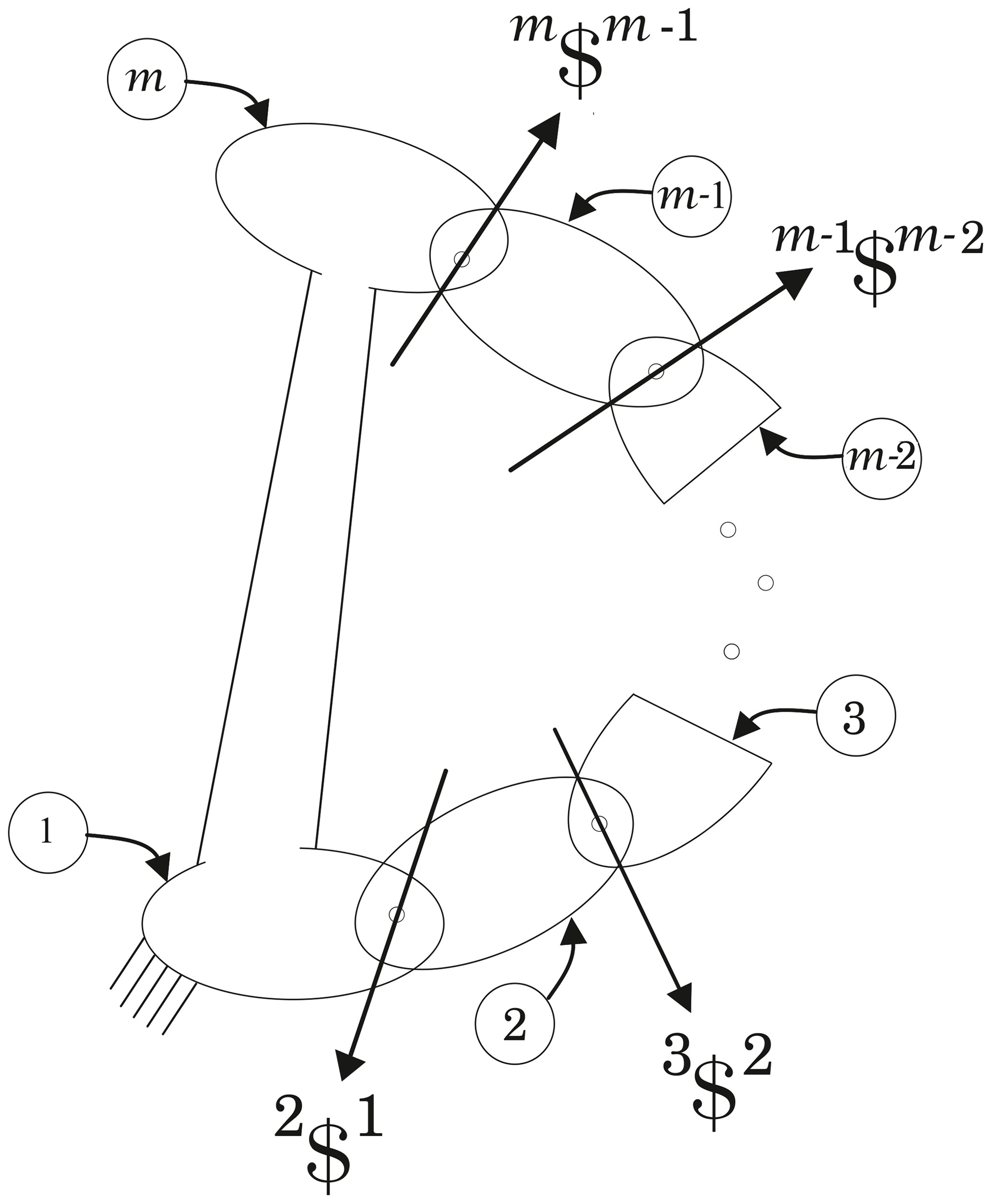
Consider the single-loop closed chain shown in Fig. 1, using recursively Eq. (3), it can be shown, see Hunt (1978), or Rico et al. (1999), that the corresponding velocity equation is given by

_{2} ω_{1}^{2} $_{O}^{1} +_{3} ω_{2}^{3} $_{O}^{2} + \dots +_{m} ω_{m - 1}^{m} $_{O}^{m - 1} = 0 .

where _j+1ω_j are the articular velocities and $^{j + 1} $_{O}^{j}$ are the corresponding screws representing the kinematic pairs. The kinematic pairs are all considered screw pairs, since revolute and prismatic pairs can be regarded as special cases of a screw pair.

https://www.mech-sci.net/11/91/2020/ms-11-91-2020-f01

Figure 1Single-loop closed chain.

Download

If link 2 is regarded as the input link, the articular velocity ₂ω₁ is known and the equation can be rewritten as

\begin{matrix} (5) & _{3} ω_{2}^{3} $_{O}^{2} + \dots +_{m} ω_{m - 1}^{m} $_{O}^{m - 1} = -_{2} ω_{1}^{2} $_{O}^{1} \end{matrix}

This is the equation employed in the solution of the velocity analysis of RCCC spatial linkages, see Sect. 3.3

If the mechanism is multi-loop, it is necessary to resort to some basics of graph theory, see Wolhart (2004), or Müller (2018). As an example, Fig. 2 shows the directed graph associated with the single flyer planar mechanism shown in Fig. 3. The nodes of the graph correspond to the links, while the edges correspond to the kinematic pairs, indicated by the instantaneous center of velocity of the revolute.

https://www.mech-sci.net/11/91/2020/ms-11-91-2020-f02

Figure 2Directed graph of the single flyer planar mechanism.

Download

https://www.mech-sci.net/11/91/2020/ms-11-91-2020-f03

Figure 3Single flyer planar mechanism.

Download

The multi-loop mechanism has three independent loops. However, there are other selections besides those shown in Fig. 2. In this case, the direction of loop I is clockwise, and the directions of the kinematic pairs in this loop are such that coincide with the direction of the loop. For the remaining loops, it is impossible to choose the direction of the kinematic pairs in such a way that all of them coincide with the direction of the loop, see Wolhart (2004). Basically, if the direction loop's edge coincide with the direction of the loop, the sign of the term in the equation is positive, otherwise the sign is negative. Therefore, the velocity equations for the single flyer planar mechanism shown in Fig. 3 are given by

\begin{matrix} (6) & \begin{aligned} _{2} ω_{1}^{2} $_{O}^{1} +_{3} ω_{2}^{3} $_{O}^{2} +_{4} ω_{3}^{4} $_{O}^{3} +_{4} ω_{1}^{4} $_{O}^{1} & = 0 \\ _{5} ω_{2}^{5} $_{O}^{2} +_{8} ω_{5}^{8} $_{O}^{5} +_{8} ω_{6}^{8} $_{O}^{6} +_{6} ω_{3}^{6} $_{O}^{3} -_{3} ω_{2}^{3} $_{O}^{2} & = 0 \\ _{8} ω_{7}^{8} $_{O}^{7} +_{7} ω_{4}^{7} $_{O}^{4} -_{4} ω_{3}^{4} $_{O}^{3} -_{6} ω_{3}^{6} $_{O}^{3} -_{8} ω_{6}^{8} $_{O}^{6} & = 0 \end{aligned} \end{matrix}

This is the equation used in the velocity analysis of the indeterminate planar mechanism dealt with in Sect. 3.1 and it is the basic equation for solving the velocity analysis of any multi-loop mechanism.

3 Examples

This section illustrates the computation of the instantaneous screw axes, or their corresponding simplifications, of three representative linkages. In all these examples, the velocity analysis, for an arbitrary velocity of the driver link will be solved, and from the results, the velocity state of an arbitrary link k with respect to another arbitrary link j will be obtained. From these results, the corresponding instantaneous screw axis, or the instantaneous pole center, if the mechanism is an spherical one, or the instantaneous center of velocity, if the mechanism is a planar one, will be easily obtained.

3.1 Indeterminate planar mechanism

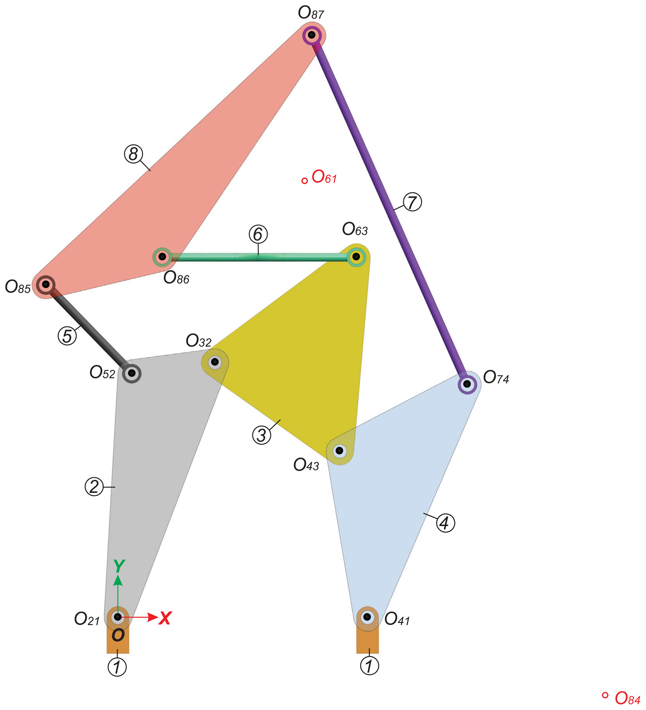
Consider the mechanism shown in Fig. 3, proposed by Klein (1917), and known as eight-bar single flyer linkage. Klein (1917) himself determined all the secondary centers using his trial and error method. Foster and Pennock (2005), and Di Gregorio (2008 b), also solved all the secondary centers. The mechanism has 4 ternary links and 4 binary links, and 10 revolute pairs. The mechanism is a trivial one, and its mobility, F, can be computed using the Grübler criterion as

F = 3 (N - 1) - 2 P_{I} = 3 (8 - 1) - 2 (10) = 1 .

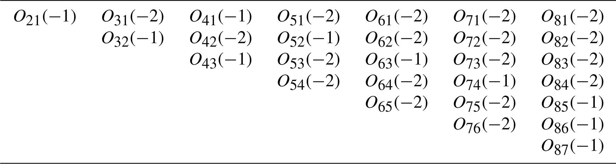
where N is the number of links, and P_I is the number of kinematic pairs of class 1, revolute pairs are precisely of class 1. The 28 instantaneous centers of velocity are shown in Table 1, where the number (−1) indicates that the instantaneous center is a primary one, while (−2) indicates that the instantaneous center is a secondary one. It should be noted that the instantaneous centers of velocity O₃₁ and O₄₂ can be easily determined using the Aronhold-Kennedy theorem. However, the remaining secondary centers can not be obtained using the theorem. Furthermore, it should be noted that, for this planar mechanism, the usual convention of denoting an instantaneous center as O_ji, where j>i has been used. This convention was also extrapolated to the infinitesimal screws.

Table 1Instantaneous centers of velocity associated with the single flyer linkage.

Download Print Version | Download XLSX

In order to carry out the velocity analysis, it is necessary to determine the screws associated with the kinematic pairs, all of them revolute pairs, with respect to the origin of the coordinate system, O. For that purpose, it is necessary to find a unit vector along the direction of the rotation axes², the Z axis, given by $u = {[\begin{array}{ccc} 0 & 0 & 1 \end{array}]}^{T}$ and the position vectors of points located along the revolute axes, with respect to the origin of the coordinate system, O, those position vectors are given in terms of an unspecified arbitrary unit of length

\begin{array}{ll} r_{21} = {[\begin{array}{ccc} 0 & 0 & 0 \end{array}]}^{T}, & r_{32} = {[\begin{array}{ccc} 70 & 184 & 0 \end{array}]}^{T}, \\ r_{43} = {[\begin{array}{ccc} 160 & 120 & 0 \end{array}]}^{T}, & r_{41} = {[\begin{array}{ccc} 180 & 0 & 0 \end{array}]}^{T}, \\ r_{52} = {[\begin{array}{ccc} 10 & 176 & 0 \end{array}]}^{T}, & r_{85} = {[\begin{array}{ccc} - 52 & 240 & 0 \end{array}]}^{T} \\ r_{86} = {[\begin{array}{ccc} 32 & 260 & 0 \end{array}]}^{T}, & r_{63} = {[\begin{array}{ccc} 172 & 260 & 0 \end{array}]}^{T}, \\ r_{87} = {[\begin{array}{ccc} 140 & 420 & 0 \end{array}]}^{T}, & r_{74} = {[\begin{array}{ccc} 252 & 168 & 0 \end{array}]}^{T} . \end{array}

where the subscripts indicate the kinematic pair associated with the position vectors.

The screws associated with the kinematic pairs, with respect to the origin, O, – again, due to space restrictions only the non-zero elements, the z component of the angular velocity, and the x and y components of the origin traslational velocity are indicated – are given by

\begin{array}{ll} ^{2} $_{O}^{1} = {[\begin{array}{ccc} 1; & 0 & 0 \end{array}]}^{T}, & ^{3} $_{O}^{2} = {[\begin{array}{ccc} 1; & 184 & - 70 \end{array}]}^{T}, \\ ^{4} $_{O}^{3} = {[\begin{array}{ccc} 1; & 120 & - 160 \end{array}]}^{T}, & ^{4} $_{O}^{1} = {[\begin{array}{ccc} 1; & 0 & - 180 \end{array}]}^{T}, \\ ^{5} $_{O}^{2} = {[\begin{array}{ccc} 1; & 176 & - 10 \end{array}]}^{T}, & ^{8} $_{O}^{5} = {[\begin{array}{ccc} 1; & 240 & 52 \end{array}]}^{T}, \\ ^{8} $_{O}^{6} = {[\begin{array}{ccc} 1; & 260 & - 32 \end{array}]}^{T}, & ^{6} $_{O}^{3} = {[\begin{array}{ccc} 1; & 260 & - 172 \end{array}]}^{T}, \\ ^{8} $_{O}^{7} = {[\begin{array}{ccc} 1; & 420 & - 140 \end{array}]}^{T}, & ^{7} $_{O}^{4} = {[\begin{array}{ccc} 1; & 168 & - 252 \end{array}]}^{T} . \end{array}

The semicolon indicates that the units of the first component is different from the remaining components. It will be assumed that the input link is link 2, and ₂ω₁=5 rad s⁻¹ is in counterclockwise sense. Solving the system of equations given by Eq. (6), the solutions are given by

\begin{array}{lll} _{3} ω_{2} = - \frac{1350}{119}, & _{4} ω_{3} = \frac{2070}{119}, & _{4} ω_{1} = - \frac{1315}{119}, \\ _{5} ω_{2} = - \frac{31 361 850}{2 420 341}, & _{8} ω_{5} = \frac{27 380 700}{2 420 341}, & _{8} ω_{6} = - \frac{17 515 170}{1 540 217}, \\ _{6} ω_{3} = \frac{28 331 370}{16 942 387}, & _{8} ω_{7} = - \frac{116 131 140}{16 942 387}, & _{7} ω_{4} = \frac{246 507 750}{16 942 387} . \end{array}

All the results are given in rad s⁻¹, if the sign is positive the angular velocity is counterclockwise and if the sign is negative the angular velocity is clockwise.

Once the velocity analysis has been completed the velocity states between two arbitrary links can be computed and the corresponding instantaneous screw axes can be determined. Due to space considerations, only a few instantaneous velocity centers will be computed; for example:

First Case. Instantaneous center of velocity O₆₁, determine the velocity state $^{1} V_{O}^{6}$ as
$\begin{array}{l} ^{1} V_{O}^{6} & =^{1} V_{O}^{2} +^{2} V_{O}^{5} +^{5} V_{O}^{8} +^{8} V_{O}^{6} \\ =_{2} ω_{1}^{2} $_{O}^{1} +_{5} ω_{2}^{5} $_{O}^{2} +_{8} ω_{5}^{8} $_{O}^{5} +_{8} ω_{6}^{8} $_{O}^{6} \\ = 5 [\begin{array}{c} 1; \\ 0 \\ 0 \end{array}] - \frac{31 361 850}{2 420 341} [\begin{array}{c} 1; \\ 176 \\ - 10 \end{array}] \\ + \frac{27 380 700}{2 420 341} [\begin{array}{c} 1; \\ 240 \\ 52 \end{array}] - \frac{17 515 170}{1 540 217} [\begin{array}{c} 1; \\ 260 \\ - 32 \end{array}] \\ = [\begin{array}{c} - \frac{135 822 985}{16 942 387}; \\ - \frac{42 731 609 400}{16 942 387} \\ \frac{426 214 980}{394 009} \end{array}] \\ = - \frac{135 822 985}{16 942 387} [\begin{array}{c} 1; \\ \frac{8 546 321 880}{27 164 597} \\ - \frac{3 665 448 828}{27 164 597} \end{array}] =_{1} ω_{6}^{1} $ {_{O}}^{6} \end{array}$
Therefore
$^{1} $ {_{O}}^{6} = {[\begin{array}{ccc} 1; & \frac{8 546 321 880}{27 164 597} & - \frac{3 665 448 828}{27 164 597} \end{array}]}^{T}$
Comparing this result with that of Eq. (2), and resorting to the triple vector identity of
$\begin{matrix} (7) & \begin{aligned} ^{A} s^{B} \times (r_{P / O} \times^{A} s^{B}) & = r_{P / O} (^{A} s^{B} \cdot^{A} s^{B}) \\ -^{A} s^{B} (^{A} s^{B} \cdot r_{P / O}) = r_{P / O}, \end{aligned} \end{matrix}$
since r_P∕O and ^As^B are perpendicular, the location of the instantaneous velocity center O₆₁ is given by
$\begin{matrix} (8) & r_{61} = {[\begin{array}{ccc} \frac{3 665 448 828}{27 164 597} & \frac{8 546 321 880}{27 164 597} & 0 \end{array}]}^{T} . \end{matrix}$
Second Case. Instantaneous center of velocity O₈₄, determine the velocity state $^{8} V_{O}^{4}$ as
$\begin{array}{l} ^{8} V_{O}^{4} & =^{8} V_{O}^{7} +^{7} V_{O}^{4} =_{8} ω_{7}^{8} $_{O}^{7} +_{7} ω_{4}^{7} $_{O}^{4} \\ = - \frac{11 6131 140}{16 942 387} [\begin{array}{c} 1; \\ 420 \\ - 140 \end{array}] + \frac{246 507 750}{16 942 387} [\begin{array}{c} 1; \\ 168 \\ - 252 \end{array}] \\ = [\begin{array}{c} \frac{18 625 230}{2 420 341}; \\ - \frac{1 051 682 400}{2 420 341} \\ - \frac{6 551 656 200}{2 420 341} \end{array}] = \frac{18 625 230}{2 420 341} [\begin{array}{c} 1; \\ - \frac{11 685 360}{206 947} \\ - \frac{72 796 180}{206 947} \end{array}] \end{array}$
From these results, the location of the instantaneous velocity center O₈₄ is given by
$r_{84} = {[\begin{array}{ccc} \frac{72 796 180}{206 947} & - \frac{11 685 360}{206 947} & 0 \end{array}]}^{T}$

The locations of the instantaneous velocity centers O₆₁ and O₈₄ are also shown in Fig. 3.

3.2 Indeterminate spherical mechanism

Consider the multi-loop spherical mechanism proposed by Zarkandi (2013), and denoted as a double butterfly spherical mechanism with a sliding pair, shown in Fig. 4. This is a completely indeterminate mechanism and its mobility can be easily computed using the Kutzbach-Grübler criterion so that F=1. The 28 instantaneous axes of velocity of the spherical mechanism are shown in Table 2, where the number (−1) indicates that the axis is primary – there are 10 primary centers – while the number (−2) indicates that the axis is secondary.

Table 2Instantaneous axes of velocity associated with the indeterminate spherical mechanism.

Download Print Version | Download XLSX

It should be noted that, unlike the planar mechanism, here the subscripts associated with the primary instantaneous axes of velocity are chosen in the way that makes simpler to understand the required velocity analysis equations.

https://www.mech-sci.net/11/91/2020/ms-11-91-2020-f04

Figure 4Indeterminate spherical mechanism.

Download

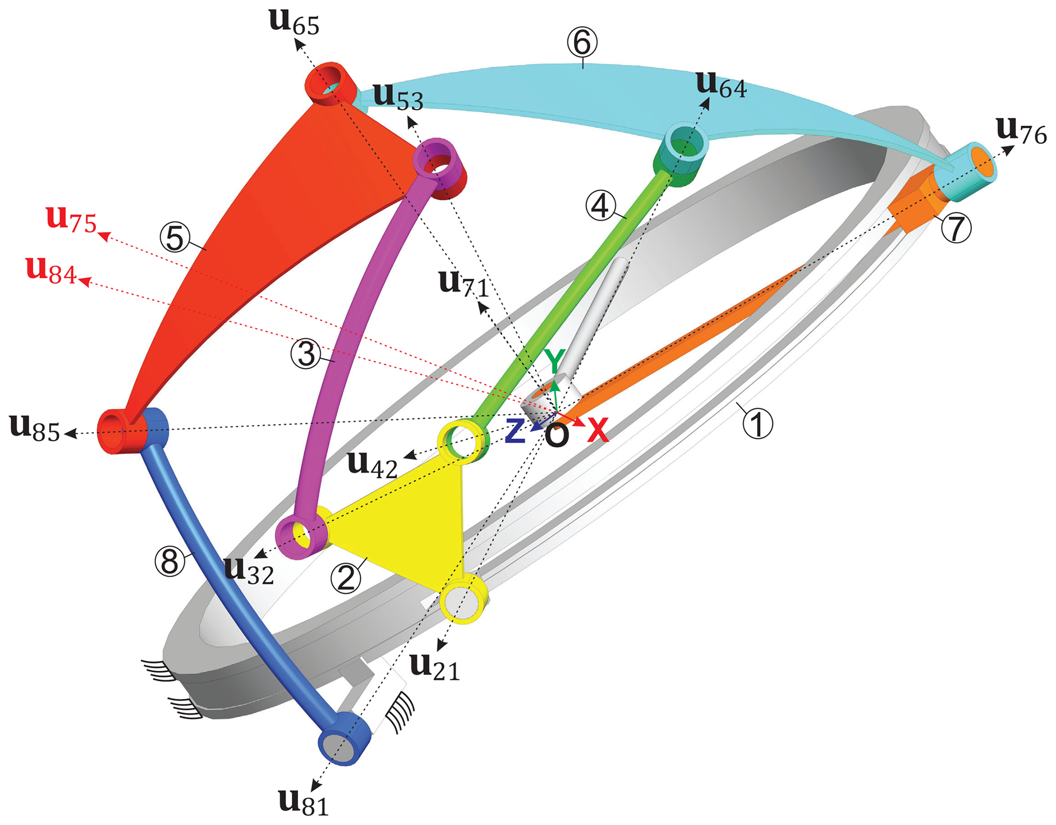
Figure 5 shows the directed graph of the spherical mechanism. The Figure also shows three independent loops that can be obtained from the mechanism, in these cases all the loops are positive in counterclockwise. Furthermore, the directions of the kinematic pairs can be established so that the equations necessary to solve the velocity analysis of the mechanism shown in Fig. 4 are given by Eq. (9). It should be noted that if the origin, O, of the coordinate system is located in the common center of all the spheres, the velocity of the origin and the translational velocity components are always zero and do not need to be considered. Therefore, the velocity equations that involve the corresponding screws are reduced to the equations involving only the unit vectors associated with the corresponding angular velocities.

https://www.mech-sci.net/11/91/2020/ms-11-91-2020-f05

Figure 5Directed graph of the single flyer spherical mechanism.

Download

\begin{matrix} (9) & \begin{aligned} _{2} ω_{1} u_{21} +_{3} ω_{2} u_{32} +_{5} ω_{3} u_{35} +_{8} ω_{5} u_{85} +_{8} ω_{1} u_{81} & = 0 \\ -_{3} ω_{2} u_{32} -_{5} ω_{3} u_{53} -_{6} ω_{5} u_{65} -_{6} ω_{4} u_{64} -_{4} ω_{2} u_{42} & = 0 \\ _{7} ω_{1} u_{71} +_{7} ω_{6} u_{76} +_{6} ω_{4} u_{64} +_{4} ω_{2} u_{42} -_{2} ω_{1} u_{21} & = 0 \end{aligned} \end{matrix}

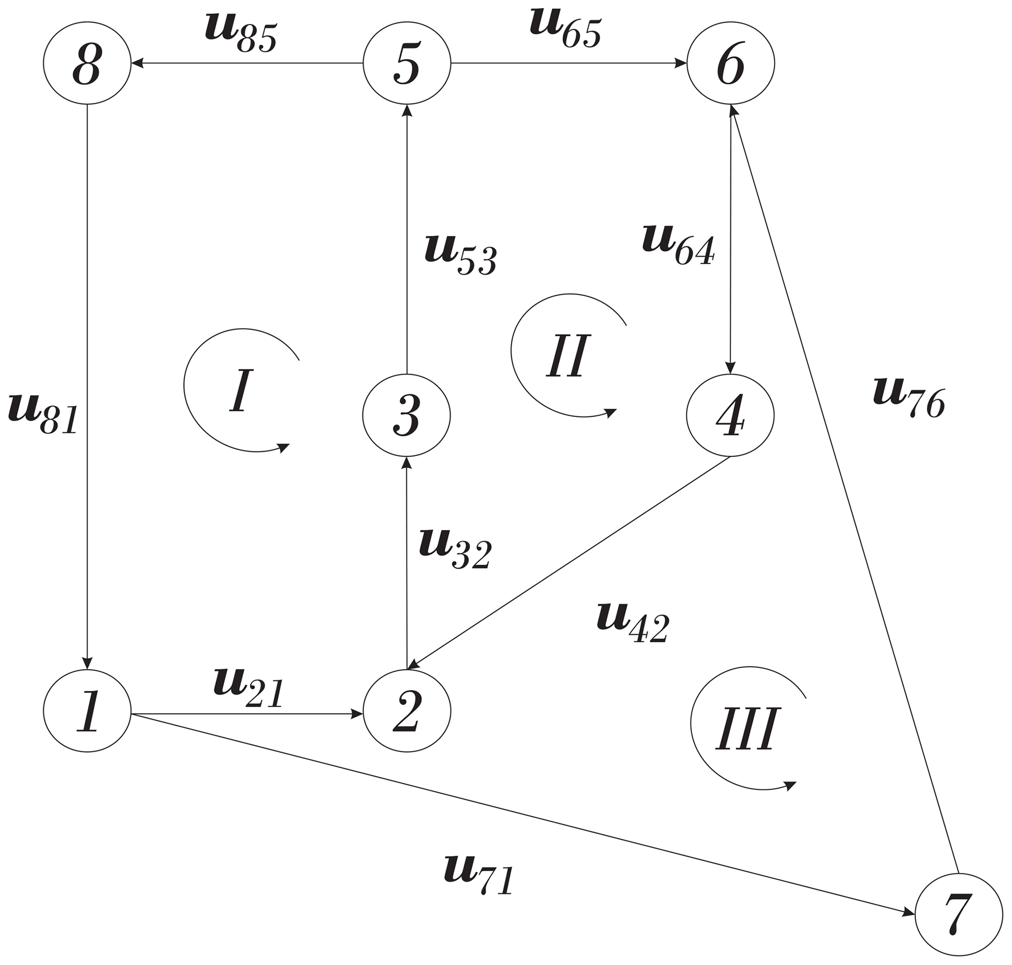
where the unit vectors associated with the primary instantaneous axes of velocity are given by

\begin{array}{ll} u_{21} = {[\begin{array}{ccc} \frac{2}{3} & \frac{1}{3} & \frac{2}{3} \end{array}]}^{T}, & u_{32} = {[\begin{array}{ccc} \frac{\sqrt{6}}{6} & \frac{\sqrt{6}}{6} & \frac{\sqrt{6}}{3} \end{array}]}^{T}, \\ u_{53} = {[\begin{array}{ccc} \frac{3}{5 \sqrt{5}} & \frac{2}{\sqrt{5}} & \frac{4}{5 \sqrt{5}} \end{array}]}^{T}, & u_{85} = {[\begin{array}{ccc} 0 & \frac{1}{\sqrt{5}} & \frac{2}{\sqrt{5}} \end{array}]}^{T}, \\ u_{81} = {[\begin{array}{ccc} \frac{1}{2} & 0 & \frac{\sqrt{3}}{2} \end{array}]}^{T}, & u_{42} = {[\begin{array}{ccc} \frac{\sqrt{3}}{3} & \frac{\sqrt{3}}{3} & \frac{\sqrt{3}}{3} \end{array}]}^{T}, \\ u_{64} = {[\begin{array}{ccc} \frac{1}{2} & \frac{\sqrt{3}}{2} & 0 \end{array}]}^{T}, & u_{65} = {[\begin{array}{ccc} 0 & \frac{12}{13} & \frac{5}{13} \end{array}]}^{T}, \\ u_{76} = {[\begin{array}{ccc} \frac{\sqrt{3}}{3} & \frac{\sqrt{3}}{3} & - \frac{\sqrt{3}}{3} \end{array}]}^{T}, & u_{71} = {[\begin{array}{ccc} - \frac{59}{100} & \frac{39}{50} & \frac{1}{5} \end{array}]}^{T} . \end{array}

Assuming that ₂ω₁=10 rad s⁻¹ is counterclockwise, the results for the articular velocities involved in Eq. (9) are – the results where obtained in Maple© in an exact form, however the radical expressions are too unwieldy to be shown here – instead only decimal approximations are shown.

\begin{array}{ll} _{3} ω_{2} = - 10.79933 rad s^{- 1}, & _{5} ω_{3} = - 2.06279 rad s^{- 1}, \\ _{8} ω_{5} = 6.53041 rad s^{- 1}, & _{8} ω_{1} = - 3.40871 rad s^{- 1}, \\ _{6} ω_{5} = 3.86346 rad s^{- 1}, & _{6} ω_{4} = - 6.21473 rad s^{- 1}, \\ _{7} ω_{1} = - 0.77268 rad s^{- 1}, & _{7} ω_{6} = 2.162413 rad s^{- 1}, \\ _{4} ω_{2} = 13.97708 rad s^{- 1} . \end{array}

From these results it is straightforward to compute the velocity state between two arbitrary links of the spherical mechanisms and eventually determine the corresponding instantaneous axis of velocity. For example:

First Case. Instantaneous axis of velocity u₅₇, determine the angular velocity $^{5} V_{O}^{7}$ as
$\begin{array}{l} ^{7} ω^{5} & =^{6} ω^{5} +^{7} ω^{6} =_{6} ω_{5} u_{65} -_{7} ω_{6} u_{76} \\ = 3.86346 {[\begin{array}{ccc} 0 & \frac{12}{13} & \frac{5}{13} \end{array}]}^{T} \\ - 2.162413 {[\begin{array}{ccc} \frac{\sqrt{3}}{3} & \frac{\sqrt{3}}{3} & - \frac{\sqrt{3}}{3} \end{array}]}^{T} \\ = {[\begin{array}{ccc} - 1.248469 & 2.31780 & 2.73441 \end{array}]}^{T} \\ = 3.79577 {[\begin{array}{ccc} - 0.3289136 & 0.6106342 & 0.7203908 \end{array}]}^{T} \end{array}$
From these results, the instantaneous axis of velocity u₇₅ is given by
$u_{75} = {[\begin{array}{ccc} - 0.3289136 & 0.6106342 & 0.7203908 \end{array}]}^{T} .$
Second Case. Instantaneous axis of velocity u₄₈, determine the angular velocity $^{4} V_{O}^{8}$ as
$\begin{array}{l} ^{4} ω^{8} & =^{4} ω^{6} +^{6} ω^{5} +^{5} ω^{8} = -_{6} ω_{4} u_{64} -_{5} ω_{6} u_{65} +_{5} ω_{8} u_{85} \\ = 6.21473 {[\begin{array}{ccc} \frac{1}{2} & \frac{\sqrt{3}}{2} & 0 \end{array}]}^{T} - 3.86346 {[\begin{array}{ccc} 0 & \frac{12}{13} & \frac{5}{13} \end{array}]}^{T} \\ + 6.53041 {[\begin{array}{ccc} 0 & \frac{1}{\sqrt{5}} & \frac{2}{\sqrt{5}} \end{array}]}^{T} \\ = {[\begin{array}{ccc} 3.107365 & 4.736331 & 4.355030 \end{array}]}^{T} \\ = 7.145266 {[\begin{array}{ccc} 0.434884 & 0.662862 & 0.609498 \end{array}]}^{T} \end{array}$
From these results, the instantaneous axis of velocity u₈₄ is given by
$u_{84} = {[\begin{array}{ccc} 0.434884 & 0.662862 & 0.609498 \end{array}]}^{T} .$
The unit vectors representing u₇₅ and u₈₄ are also shown in Fig. 4.

3.3 Spatial mechanism

Consider the RCCC spatial mechanism shown in Fig. 6, where the kinematic pair between links 1 and 2 is a revolute and the remaining pairs are cylindrical. The mechanism is a trivial one and its mobility F=1 can be computed using the Kutzbach-Grübler criterion. The unit vectors associated with the revolute axis and the cylindrical pairs axes are given by

\begin{array}{l} u_{21} & = {[\begin{array}{ccc} - \frac{\sqrt{30}}{6} & \frac{\sqrt{30}}{15} & \frac{\sqrt{30}}{30} \end{array}]}^{T}, \\ u_{32 a} = u_{32 b} & = {[\begin{array}{ccc} \frac{4 \sqrt{29}}{29} & \frac{3 \sqrt{29}}{29} & - \frac{2 \sqrt{29}}{29} \end{array}]}^{T}, \\ u_{43 a} = u_{43 b} & = {[\begin{array}{ccc} \frac{12 \sqrt{161}}{161} & \frac{\sqrt{161}}{161} & \frac{4 \sqrt{161}}{161} \end{array}]}^{T}, \\ u_{41 a} = u_{41 b} & = {[\begin{array}{ccc} \frac{3 \sqrt{22}}{22} & \frac{\sqrt{22}}{11} & \frac{3 \sqrt{22}}{22} \end{array}]}^{T} . \end{array}

Similarly, the position vectors of points along the kinematic pairs with respect to the origin, O, are given by

\begin{array}{ll} r_{21} = {[\begin{array}{ccc} 0 & 0 & 0 \end{array}]}^{T}, & r_{32} = {[\begin{array}{ccc} 246 & 388 & - 176 \end{array}]}^{T}, \\ r_{43} = {[\begin{array}{ccc} 580 & 224 & 175 \end{array}]}^{T}, & r_{41} = {[\begin{array}{ccc} 671 & 27 & - 28 \end{array}]}^{T} . \end{array}

The screws associated with the kinematic pairs of the RCCC mechanism, where each cylindrical pair has two screws associated with the pair, are given by

\begin{array}{l} ^{2} $_{O}^{1} & = {[\begin{array}{cccccc} - \frac{\sqrt{30}}{6} & \frac{\sqrt{30}}{15} & \frac{\sqrt{30}}{30}; & 0 & 0 & 0 \end{array}]}^{T}, \\ ^{3 a} $_{O}^{2} & = {[\begin{array}{cccccc} \frac{4}{\sqrt{29}} & \frac{3}{\sqrt{29}} & - \frac{2}{\sqrt{29}}; & - \frac{248}{\sqrt{29}} & - \frac{212}{\sqrt{29}} & - \frac{814}{\sqrt{29}} \end{array}]}^{T}, \\ ^{3 b} $_{O}^{2} & = {[\begin{array}{cccccc} 0 & 0 & 0; & \frac{4}{\sqrt{29}} & \frac{3}{\sqrt{29}} & - \frac{2}{\sqrt{29}} \end{array}]}^{T}, \\ ^{4 a} $_{O}^{3} & = {[\begin{array}{cccccc} \frac{12}{\sqrt{161}} & \frac{1}{\sqrt{161}} & \frac{4}{\sqrt{161}}; & \frac{103 \sqrt{7}}{\sqrt{23}} & - \frac{220}{\sqrt{161}} & - \frac{2108}{\sqrt{161}} \end{array}]}^{T}, \\ ^{4 b} $_{O}^{3} & = {[\begin{array}{cccccc} 0 & 0 & 0; & \frac{12}{\sqrt{161}} & \frac{1}{\sqrt{161}} & \frac{4}{\sqrt{161}} \end{array}]}^{T}, \\ ^{4} $_{O}^{1 a} & = {[\begin{array}{cccccc} \frac{3}{\sqrt{22}} & \frac{\sqrt{22}}{11} & \frac{3}{\sqrt{22}}; & \frac{137}{\sqrt{22}} & - \frac{2097}{\sqrt{22}} & \frac{1261}{\sqrt{22}} \end{array}]}^{T}, \\ ^{4} $_{O}^{1 b} & = {[\begin{array}{cccccc} 0 & 0 & 0; & \frac{3}{\sqrt{22}} & \frac{\sqrt{22}}{11} & \frac{3}{\sqrt{22}} \end{array}]}^{T} . \end{array}

https://www.mech-sci.net/11/91/2020/ms-11-91-2020-f06

Figure 6The RCCC spatial mechanism.

Download

The velocity analysis equation is given by

\begin{matrix} (10) & \begin{aligned} _{3 a} ω_{2}^{3 a} $_{O}^{2} +_{3 b} v_{2}^{3 b} $_{O}^{2} +_{4 a} ω_{3}^{4 a} $_{O}^{3} +_{4 b} v_{3}^{4 b} $_{O}^{3} \\ +_{4} ω_{1 a}^{4} $_{O}^{1 a} +_{4} v_{1 b}^{4} $_{O}^{1 b} = -_{2} ω_{1}^{2} $_{O}^{1} \end{aligned} \end{matrix}

where ₂ω₁=10 rad s⁻¹, the results of the velocity analysis are:

\begin{array}{ll} _{3 a} ω_{2} = - \frac{\sqrt{870}}{201} rad s^{- 1}, & _{3 b} v_{2} = - \frac{3 029 587 \sqrt{870}}{8978} u . l . s^{- 1}, \\ _{4 a} ω_{3} = \frac{17 \sqrt{4830}}{67} rad s^{- 1}, & _{4 b} v_{3} = \frac{898 707 \sqrt{4830}}{8978} u . l . s^{- 1}, \\ _{4} ω_{1 a} = - \frac{91 \sqrt{660}}{201} rad s^{- 1}, & _{4} v_{1 b} = \frac{118 604 \sqrt{660}}{13 467} u . l . s^{- 1} . \end{array}

From these results, it is possible to determine the velocity states of the different links relative to the other links, and from these velocity states the corresponding instantaneous screw axes, ISA will be determined. One special and simplest case is the ISA of the relative movement of link 2 to link 1. Since its velocity state is given by

^{1} V_{O}^{2} =_{2} ω_{1}^{2} $_{O}^{1}

Therefore, the instantaneous screw axis ISA of link 2 with respect to link 1 is given by

\begin{matrix} (11) & ^{2} $_{O}^{1} = \frac{1}{_{2} ω_{1}}^{2} V_{O}^{1} = {[\begin{array}{cccccc} - \frac{\sqrt{30}}{6} & \frac{\sqrt{30}}{15} & \frac{\sqrt{30}}{30}; & 0 & 0 & 0 \end{array}]}^{T} . \end{matrix}

The next task is to find the ISA of the relative movement of link 3 to link 2. It should be noted that the kinematic pair between links 2 and 3 is a cylindrical pair, thus at the outset it seems that there is not a unique ISA; however, after carrying out the velocity analysis the joint velocities are uniquely determined and the velocity state of link 3 with respect to link 2 is given by

\begin{array}{l} ^{2} V_{O}^{3} & =_{3 a} ω_{2}^{3 a} $_{O}^{2} +_{3 b} v_{2}^{3 b} $_{O}^{2} \\ = \frac{- \sqrt{29} \sqrt{30}}{201} {[\begin{array}{cccccc} \frac{4}{\sqrt{29}} & \frac{3}{\sqrt{29}} & \frac{- 2}{\sqrt{29}}; & \frac{- 248}{\sqrt{29}} & \frac{- 212}{\sqrt{29}} & \frac{- 814}{\sqrt{29}} \end{array}]}^{T} \\ \frac{- 3 029 587 \sqrt{29} \sqrt{30}}{8978} {[\begin{array}{cccccc} 0 & 0 & 0; & \frac{4}{\sqrt{29}} & \frac{3}{\sqrt{29}} & \frac{- 2}{\sqrt{29}} \end{array}]}^{T} \\ = \frac{\sqrt{870}}{201} {[\begin{array}{cccccc} \frac{- 4}{\sqrt{29}} & \frac{- 3}{\sqrt{29}} & \frac{2}{\sqrt{29}}; & \frac{18 160 906}{\sqrt{67}} & \frac{27 237 875}{\sqrt{134}} & \frac{- 9 143 299}{\sqrt{67}} \end{array}]}^{T} \end{array}

Therefore the instantaneous screw axes of the relative movement of link 3 with respect to link 2 is given by

\begin{matrix} (12) & ^{3} $_{O}^{2} = {[\begin{array}{ccc} \frac{- 4}{\sqrt{29}} & \frac{- 3}{\sqrt{29}} & \frac{2}{\sqrt{29}}; \\ \frac{18 160 906}{\sqrt{67}} & \frac{27 237 875}{\sqrt{134}} & \frac{- 9 143 299}{\sqrt{67}} \end{array}]}^{T} . \end{matrix}

The results of Eqs. (11) and (12) verify the data employed in the setting up of this problem.

Now, the the ISA of the relative movement of link 3 to link 1 will be determined. It follows that

\begin{array}{l} ^{1} V_{O}^{3} & =^{1} V_{O}^{2} +^{2} V_{O}^{3} =_{2} ω_{1}^{2} $_{O}^{1} +_{3 a} ω_{2}^{3 a} $_{O}^{2} +_{3 b} v_{2}^{3 b} $_{O}^{2} \\ = 10 {[\begin{array}{cccccc} - \frac{\sqrt{30}}{6} & \frac{\sqrt{30}}{15} & \frac{\sqrt{30}}{30}; & 0 & 0 & 0 \end{array}]}^{T} \\ - \frac{\sqrt{29} \sqrt{30}}{201} {[\begin{array}{cccccc} \frac{4}{\sqrt{29}} & \frac{3}{\sqrt{29}} & \frac{- 2}{\sqrt{29}}; & \frac{- 248}{\sqrt{29}} & \frac{- 212}{\sqrt{29}} & \frac{- 814}{\sqrt{29}} \end{array}]}^{T} \\ - \frac{3 029 587 \sqrt{29} \sqrt{30}}{8978} {[\begin{array}{cccccc} 0 & 0 & 0; & \frac{4}{\sqrt{29}} & \frac{3}{\sqrt{29}} & \frac{- 2}{\sqrt{29}} \end{array}]}^{T} \\ = \frac{\sqrt{4 105 290}}{201} {[\begin{array}{ccc} \frac{- 3 \sqrt{113}}{\sqrt{1211}} & \frac{131}{\sqrt{136 843}} & \frac{69}{\sqrt{136 843}}; \\ \frac{- 18 160 906}{67 \sqrt{136 843}} & - \frac{3 891 125 \sqrt{136 843}}{2 619 566} & \frac{9 143 299}{67 \sqrt{136 843}} \end{array}]}^{T} . \end{array}

Therefore, the angular velocity of link 3 with respect to link 1 is given

_{3} ω_{1} = \frac{\sqrt{4 105 290}}{201} rad s^{- 1},

and the ISA associated with the movement of link 3 with respect to link 1 is given

^{3} $_{O}^{1} = {[\begin{array}{ccc} \frac{- 3 \sqrt{113}}{\sqrt{1211}} & \frac{131}{\sqrt{136 843}} & \frac{69}{\sqrt{136 843}}; \\ \frac{- 18 160 906}{67 \sqrt{136 843}} & - \frac{3 891 125 \sqrt{136 843}}{2 619 566} & \frac{9 143 299}{67 \sqrt{136 843}} \end{array}]}^{T}

The line associated to the screw $^{3} $_{O}^{1}$ is also shown in Fig. 6. Due to space considerations, the computation of $^{4} $_{O}^{2}$ is omitted.

4 Conclusions

This paper has shown that once the velocity analysis of an arbitrary mechanism with one degree of freedom has been carried out it is straightforward to determine the instantaneous screw axis associated with the relative movement of two arbitrary links of the mechanism, regardless the type of mechanism, whether they are single- or multi-loop, or they are determined or undetermined. However, it should be noted that in kinematics, the usual approach is to find first the instantaneous screw axis associated with two arbitrary links of the mechanism and from this knowledge to perform the mechanism's velocity analysis. An upcoming paper will analyze thoroughly this approach for arbitrary mechanisms. All the computations were carried out using Maple© and verified with Adams©.

Data availability

The complete thesis of Juan Ignacio Valderrama-Rodríguez is located in https://github.com/ibarram/Tesis-JIVR/blob/master/Tesis - JIVR.pdf (Valderrama-Rodríguez, 2020).

Author contributions

The present work originated from the Master thesis of JIVR. JMR and JJCS were the co-directors of the thesis. It can be assured that the authors worked proportionally to the thesis and the present paper.

Competing interests

The authors declare that they have no conflict of interest.

Acknowledgements

Juan Ignacio Valderrama-Rodríguez thanks the Conacyt, the Mexican National Council of Science and Technology, for the support through a grant no. 458523 to pursue a MSc degree at the Universidad of Guanajuato. The authors thank Conacyt and the Universidad of Guanajuato, through DICIS and the Mechanical Engineering Department, for their continuous support.

Financial support

This research has been supported by the Mexican National Council of Science and Technology (grant no. 458523).

Review statement

This paper was edited by Daniel Condurache and reviewed by Soheil Zarkandi and two anonymous referees.

References

Aronhold, S.: Gründzuge der Kinematischen Geometrie, Verh. d. Ver. Z. Beförderung des Gewerbefleiss in Preussen, 51, 129–155, 1872. a

Di Gregorio, R.: A novel geometric and analytic technique for the singularity analysis of one-dof planar mechanisms, Mech. Mach. Theory, 42, 1462–1483, 2007. a

Di Gregorio, R.: Determination of the instantaneous pole axes in single-Dof spherical mechanisms, Proceedings of the ASME 2008 International Design Engineering Technical Conferences & Computers and Informationn in Engineering Conference IDETC/CIE 2008, Brooklyn, N.Y. Paper DETC 2008-49084, 2008a. a

Di Gregorio, R.: An algorithm for analytically calculating the positions of the secondary instant centers of indeterminate linkages, J. Mech. Des.-T. ASME, 130, 1–9, 2008b. a, b

Di Gregorio, R.: A general algorithm for analytically determining all the instantaneous pole axis locations in single – Dof spherical mechanisms, P. I. Mech. Eng. C-J. Mec., 225, 2062–2075, 2011. a

Foster, D. E. and Pennock, G. R.: A Graphical Method to Find the Secondary Instantaneous Centers of Zero Velocity for the Double Butterfly Linkage, J. Mech. Des.-T. ASME, 125, 268–274, 2003. a

Foster, D. E. and Pennock, G. R.: Graphical methods to locate the secondary instant centers of single-degree-of-freedom indeterminate linkages, J. Mech. Des.-T. ASME, 127, 249–256, 2005. a, b

Hervé, J. M.: Analyse Structurelle des Mécanismes par Groupe des Déplacements, Mech. Mach. Theory, 13, 437–450, 1978. a

Hunt, K. H.: Kinematic Geometry of Mechanisms, Oxford, Clarendon Press, 1978. a, b

Kennedy, A. B. W.: The Mechanics of Machinery, Macmillan, London, 1886. a

Kim, M., Han, M. S., Seo, T. W., and Lee, J. W.: A New Instantaneous Center Analysis Methodology for Planar Closed Chains via Graphical Representation, Int. J. Control Autom., 14, 1528–1534, 2016. a, b, c, d, e, f, g, h, i, j

Klein, A. W.: Kinematics of Machinery, Mc-Graw Hill Book Co, New York, 1917. a, b, c, d

Kung, C. M. and Wang, L. C. T.: Analytical method for locating the secondary instant centers of indeterminate planar linkages, P. I. Mech. Eng. C-J. Mec., 223, 491–502, 2009. a

Müller, A.: Kinematic topology and constraints of multi-loop linkages, Robotica, 36, 1641–1663, 2018. a

Rico, J. M., Gallardo, J., and Duffy, J.: Screw Theory and Higher Order Kinematic Analysis of Open Serial and Closed Chains, Mech. Mach. Theory, 34, 559–586, 1999. a, b

Valderrama-Rodríguez, J. I.: Localización de los Ejes de Tornillos Instantáneos de Mecanismos Espaciales y sus Aplicaciones, available at: https://github.com/ibarram/Tesis-JIVR/blob/master/Tesis - JIVR.pdf, last access: 25 March 2020. a

Wohlhart, K.: Screw Spaces and Connectivities in Multiloop Linkages, in: On Advances in Robot Kinematics, edited by: Lenarčič, J. and Galletti, C., 97–104, Kluwer Academic Publishers, Dordrecht, 2004. a, b, c

Yan, H. S. and Hsu, M. H.: An Analytical Method for Locating Instantaneous Velocity Centers, Proceedings of the 22nd ASME Biennial Mechanisms Conference, Scottsdale, AZ, 13–16 September 1992, DE-Vol. 47, 353–359, 1992. a

Zarkandi, S.: Geometrical methods to locate secondary instantaneous poles of single – DOF indeterminate spherical mechanisms, Journal of Mechanical Engineering Transactions of Mechanical Engineering Division, The Institution of Engineers, Bangladesh, 41, 80–88, 2010. a

Zarkandi, S.: A new geometric method for singularity analysis of spherical mechanisms, Robotica, 29, 1083–1092, 2011. a

Zarkandi, S.: An Analytical Approach to Locate the Secondary Instantaneous Poles of Single-DOF Indeterminate Spherical Mechanisms, Mech. Based Des. Struc., 41, 274–292, 2013. a, b

Zhao, J. S. and Zhou, K.: A novel methodology to study the singularity of spatial parallel mechanisms, International Journal Advanced Manufacturing Technology, 23, 750–754, 2004. a

Here, Kim et al. (2016) is referring to the application of the Aronhold-Kennedy theorem.

In this contribution all vectors are column vectors; however due to space considerations they are written as the transpose of row vectors.

Articles

Short summary

The paper presents a general procedure to determine the instantaneous rotation center for planar mechanisms, or its kinematical equivalent in the case of spherical or spatial cases, from the velocity analysis of the mechanism. The procedure is based on the theoretical results of the Lie algebra, se(3), of the Euclidean group, together with the Killing and Klein forms. The paper shows that a previous contribution contains fundamental errors and it was done in order to unify the theory.