the Creative Commons Attribution 4.0 License.
the Creative Commons Attribution 4.0 License.
 | 23 Apr 2020
Code-to-code verification for thermal models of melting and solidification in a metal alloy: comparisons between a Finite Volume Method and a Finite Element Method
Anna M. V. Harley
Sagar H. Nikam
Hao Wu
Justin Quinn
Shaun McFadden
Verification, the process of checking a modelling output against a known reference model, is an important step in model development for the simulation of manufacturing processes. This manuscript provides details of a code-to-code verification between two thermal models used for simulating the melting and solidification processes in a 316 L stainless steel alloy: one model was developed using a non-commercial code and the Finite Volume Method (FVM) and the other used a commercial Finite Element Method (FEM) code available within COMSOL Multiphysics®. The application involved the transient case of heat-transfer from a point heat source into one end of a cylindrical sample geometry, thus melting and then re-solidifying the sample in a way similar to an autogenous welding process in metal fabrication. Temperature dependent material properties and progressive latent heat evolution through the freezing range of the alloy were included in the model. Both models were tested for mesh independency, permitting meaningful comparisons between thermal histories, temperature profiles and maximum temperature along the length of the cylindrical rod and melt pool depth. Acceptable agreement between the results obtained by the non-commercial and commercial models was achieved. This confidence building step will allow for further development of point-source heat models, which has a wide variety of applications in manufacturing processes.


Verification and validation are two procedures in model development that are often discussed interchangeably. However, in the context of the American Institute of Aeronautics and Astronautics (AIAA) definition (Roache, 2012), verification is the process of checking that a code's simulation output is consistent with the underlying mathematical requirements, whereas validation is the process of checking a code's simulated outputs against well-defined physical experimental results. Both steps are essential in model development, but verification precedes validation.
Verification, the focus of this manuscript, is usually performed by comparing the outputs from a numerically derived computer model to the same results from an analytical, mathematical model. Hence the computer code (with its inherent numerical artefacts) is compared to the benchmark analytical model for accuracy (Pelletier and Roache, 2000). However, analytical models are often only available for simple benchmark cases. In many instances there are no analytical solutions available to the code developer. Nevertheless, formal order of accuracy verification methods are available to investigate the convergence and whether it follows the expected order of convergence (Roache, 1998). In the case where an analytical solution is unavailable, mesh-independent numerical simulation results for identical modelling scenarios can be compared; this approach is known as code-to-code verification.
This contribution outlines a code-to-code verification where we compare the modelling outputs from two models of a stationary point heat source with a time-dependent heat input into a metal alloy of known geometry. This simulation scenario is a melting-solidification process similar to that found in welding or additive manufacturing processes. Comparisons between a non-commercial, bespoke, 1D Finite Volume Method (FVM) and a commercial 3D Finite Element Method (FEM) were conducted and are presented here. The models were produced by MATLAB® (FVM) and COMSOL Multiphysics® (FEM) respectively. Both models consider heat transfer only. The effect on temperature distribution across the sample will be investigated. A mesh sensitivity analysis was completed to ensure mesh-independent results were obtained for each modelling approach. This comparative verification study will give confidence in the modelling approaches, so that future work in the development of a 3D FEM model with a moving point heat source and layer additions can take place. This type of model will find application in welding processes or metal additive manufacturing processes.
1.1 Literature review
Verification studies, performed as part of the development process for bespoke models of solidification, are available in literature. A summary of these investigations that relate to heat transfer and phase change (solidification) are provided here.
Mooney and co-authors developed a 1D model of the Bridgman furnace process known as the Bridgman Furnace Front Tracking Model (BFFTM) (Mooney et al., 2012). The Bridgman process is a well-known, crystal growth method whereby the sample is translated through a controlled temperature gradient zone in a furnace at a known translation speed. The model used a columnar dendritic, front-tracking model for metal alloy solidification combined with a FVM approach. In order to build confidence in the BFFTM, a verification study (Mooney and McFadden, 2014) was conducted, whereby the BFFTM code was adapted to a pure material and then compared against an analytical solution of the same process (Naumann, 1982) under the same processing conditions.
A thermal model of equiaxed polycrystalline solidification, based on the Nucleation Progenitor Function (NPF) approach (McFadden et al., 2018) was applied to a microgravity experiment with a solidifying transparent analogue alloy material (Mooney et al., 2018). A formal order of accuracy verification exercise was conducted during the thermal characterisation and application of the model (Mooney et al., 2018). The observed order of accuracy during the mesh convergence study was shown to be greater than 1.96 and less than 2.0. This agreed closely with the expected order of accuracy value of 2 derived from theory. Hence, the model was verified as second order accurate.
Additionally, literature contains examples of comparisons between modelling approaches to verify results, known as code-to-code verification. For example, Pineau et al. (2018) performed an analysis of the Phase Field method versus the Cellular Automata (CA) method for columnar dendritic solidification in a succinonitrile-acetone alloy. It was concluded that the more computationally intensive and detailed Phase Field method was used to calibrate the CA method for larger scale simulations.
Battaglioli et al. (2017a, b) developed the Bridgman furnace model to include 2D axisymmetric geometries. Seredyński et al. (2017) used ANSYS Fluent® to verify the results from the 2D Bridgman model by performing a code-to-code verification. This study showed that the results from the commercial code agreed very closely with the results from the non-proprietary code for analysing transient operation of the Bridgman furnace.
The literature demonstrates that, in the absence of formal analytical solutions to well-defined modelling problems, verification of thermal simulation codes can proceed with the application formal order-of-accuracy methods or via code-to-code verification.
1.2 Aims and Objectives
The aim of the present study is to perform a code-to-code verification between two thermal models (FVM and FEM) of the transient phenomenon of melting followed by solidification. To achieve this aim, the following objectives were targeted:
-
Develop non-commercial and commercial models to simulate the heat transfer process of heating the top surface of a cylindrical 316 L stainless steel rod with a point heat source.
-
Obtain mesh independent non-commercial and commercial model results.
-
Compare the results of thermal histories, temperature distributions and peak temperatures along the length of the cylindrical rod and the melt pool depths obtained by both models.
-
Demonstrate the scenario of temperature distributions at different time intervals using the commercial model developed in COMSOL Multiphysics®.
After the introduction section, the manuscript is divided in following sections: Materials and Methods, Results, Discussion and Conclusion.
The Material and Methods section describes the development of the non-commercial and commercial models using FVM and FEM respectively. The heat equations and boundary conditions were coded using MATLAB® for the non-commercial model and simulated with COMSOL Multiphysics® v.5.4 for the commercial model. The section also outlines data related to physical process parameters for welding and thermophysical material properties for 316 L stainless steel.
The Results section provides a detailed description and comparison of the results obtained by both modelling methods.
The Discussion section provides a significant insight into the results obtained.
Finally, the Conclusion section will summarise the key findings and review the outcomes in contrast to the objectives of this study.
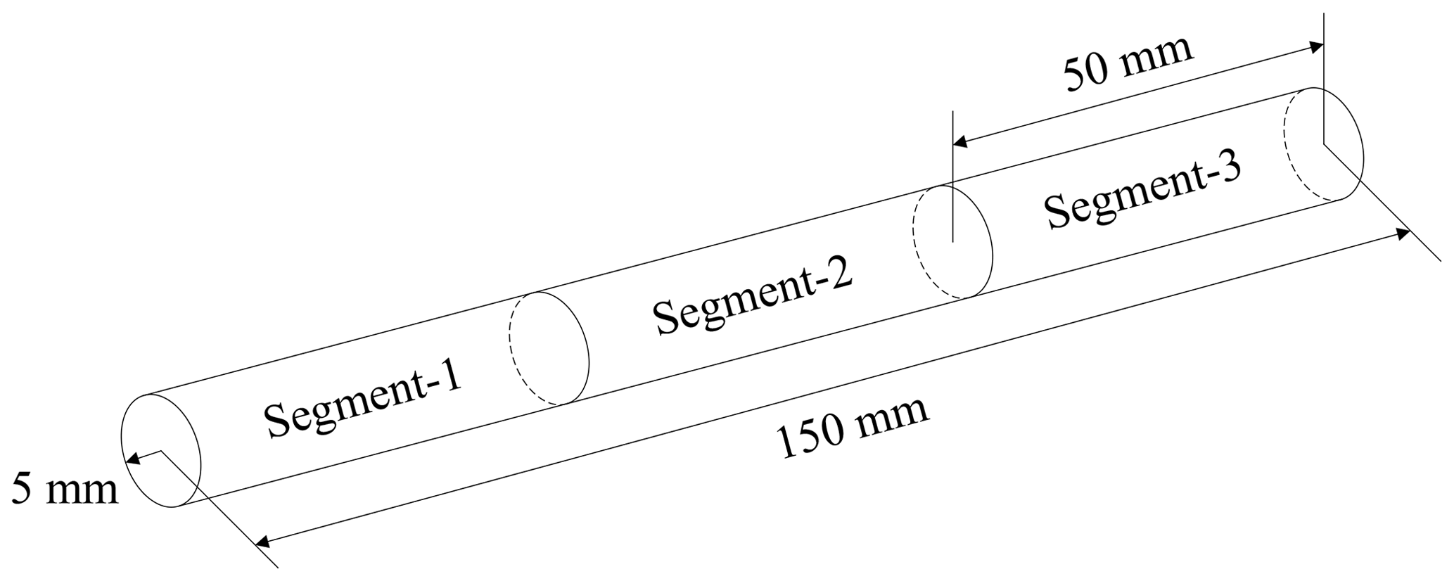
The scenario in this study is shown schematically in Fig. 1. A cylindrical sample of 316 L stainless steel is held in a crucible and is heated from one end using a point heat source. The point heat source on the left-hand side is assumed to ramp up linearly from zero to one second, reaching a maximum power value of 400 W. This maximum power is maintained until 35 s of process time has elapsed. The power is then ramped down, linearly, over the next 5 s, i.e., the power input will have returned to zero after 40 s of process time. The heat flux due to the power input is assumed to be uniformly distributed over the area on the left boundary. The cylindrical rod has a radius of 5 mm and length of 150 mm. The right-hand boundary, x=150 mm, is assumed to be adiabatic.

2.1 Non-commercial 1D code
2.1.1 Mathematical and numerical background
The heat transfer equation for the 1D model follows that given by the BFFTM (Mooney et al., 2012) but without the advection term because no translation of the sample takes place. This equation is expressed as:
where t is the time, ρ is the density of the cylindrical bar, cp is the specific heat, T is the temperature, k is the thermal conductivity, hI is the interfacial heat transfer coefficient, C is the circumference of the cylindrical bar, A is the cross-sectional area, TWall is the constant temperature of the crucible, and E is the latent heat term. An expansion of the latent heat term gives
where L is the specific latent heat and fS is the solid fraction.
The relationship between the solid fraction and temperature, T, is given as follows:
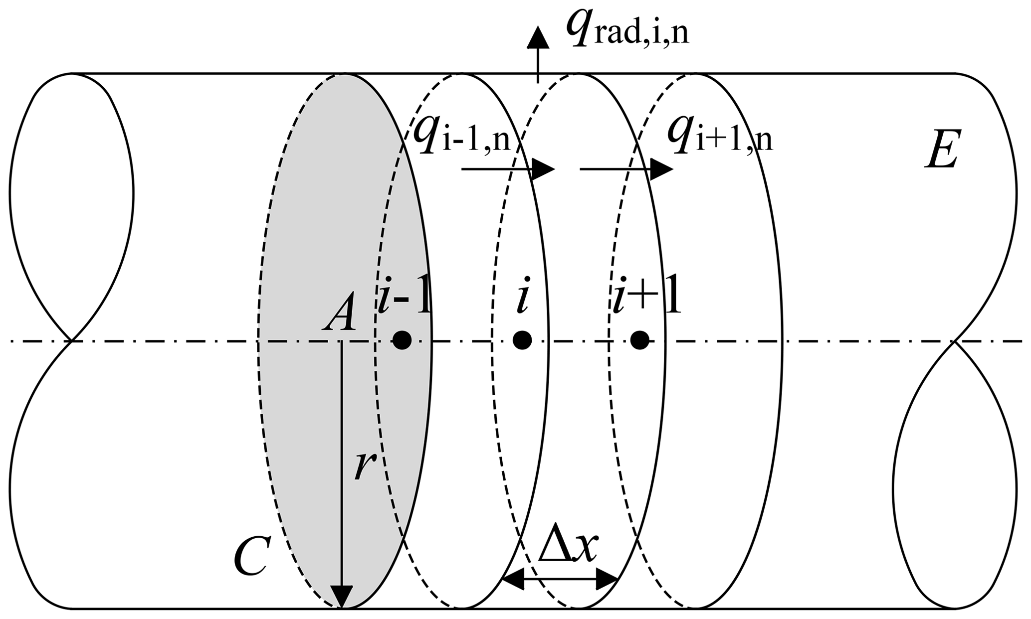
In the FVM, the geometry of the cylindrical rod is discretised with a finite number of the control volume (CVs) discs having a width of Δx. Figure 2 depicts the details of the disc shaped CV, labelled as “i” and its adjacent CVs are labelled as “i−1” and “i+1”. The solution to Eq. (1) can be implemented by considering the energy balance for CV “i” at time step “n”:
where and Ti,n, are the temperatures at the next time step “n+1” and current time step “n” of CV “i”, r is the radius of the bar, fi,n is the solid fraction, and is the radial heat loss from the side of the disc-shape CV, as indicated by Fig. 2. In this study, this is simplified as equivalent to the interfacial heat between the bar and the crucible, which can be expressed as:
The term in Eq. (4) is the interfacial heat flux of thermal diffusion from the previous CV “i−1” to CV “i”, and is the interfacial heat flux from CV “i” to the next CV “i+1”, which can be expressed as the following finite difference equations:
where , Ti,n and are the temperatures of CVs “i−1”, “i”, and “i+1” respectively at time step “n”. Inserting Eqs. (5), (6), and (7) into Eq. (4) and rearranging gives Eq. (8), which can be used to compute the temperature distribution of CV “i” at the next time step “n+1”:
where TL is the liquidus temperature and TS is the solidus temperature. This approach is known as an explicit scheme.
Latent heat “L” is only considered in the mushy zone, i.e., when the temperature of CV is greater than the solidus temperature and lower than the liquidus temperature () as indicated by Eq. (3).
Figure 3a and b shows a flowchart for the main code algorithm and subroutine which has been used in the production of the non-commercial code.
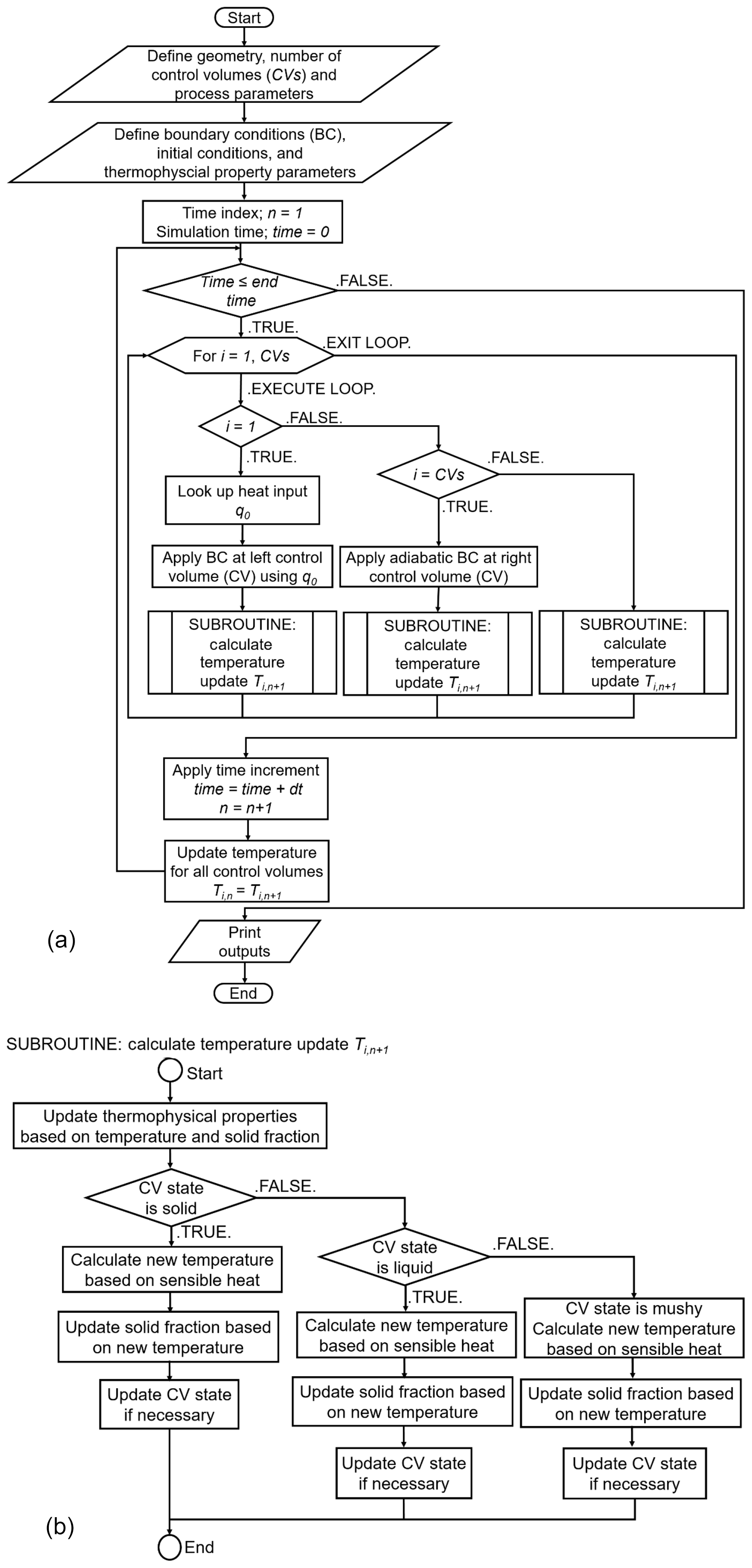
Figure 3(a) Flow chart describing the relevant steps taken within the non-commercial code. (b) Flow chart describing the relevant steps taken within subroutine of the non-commercial code.
2.2 Commercial code
COMSOL Multiphysics® v.5.4 was used to model the geometry, the dimensions of which are identical to the FVM model. Figure 4 shows how the domain was segmented into three sections, equally spaced at 50 mm. This segmentation allowed for independent meshing scenarios within each segment.
2.2.1 Modelling phase change in COMSOL Multiphysics®
Phase change in COMSOL Multiphysics® was performed using an apparent heat capacity method (COMSOL Multiphysics ® v.5.4, 2018). The inbuilt COMSOL® phase change material sub-node was used to specify the properties of the material to change from phase 1 to phase 2. In our case phase 1 was designated as solid and phase 2 was designated as liquid. In COMSOL®, the transition between the phases is assumed to occur smoothly over a temperature interval ΔT. COMSOL® accounts for the release of latent heat over the temperature interval between 2 and where Tpc is the temperature which initiates the phase change in material. During this interval, the phenomenon of phase change within the material is assigned to thermal models using a smoothed function, θ, to represent the solid fraction. Equations (9) and (10) represents the fraction of phase prior to transition.
Material properties such as density, ρ, and enthalpy, H, were updated according to the phase change taking place in that temperature interval. Equations (11) and (12) were used to accommodate this phenomenon in the COMSOL Multiphysics® model:
where, ph1 and ph2 indicate phase 1 and phase 2 of the material. Input parameters for the transition are given in Table 1. The COMSOL® phase change input parameters are related to the materials liquidus and solidus temperatures, TL and TS respectively.
Table 1Parameters and values used within the COMSOL Multiphysics® subnode.

2.2.2 The heat input
The 3D model accounted for a time-dependent power input to the left-hand boundary using a piecewise linear function. The function was set to 0 W at 0 s with full ramping up of the power from the heat source after 1 s. Thereafter, the power maintained its maximum value, 400 W, for the next 34 s. After 35 s of process time, the power ramped down to 0 W over 5 s. The simulation ran for 100 s (140 s of process time). A general stationary inward heat flux, q0, has been considered in the present model. This adds to the total flux across selected boundaries.
The inward heat flux, q0, may be calculated from the power input as:
where, q0 is the general inward heat flux, P is the power of heat source from the piecewise linear function described earlier and A is the cross-sectional area of the cylindrical rod. A peak q0 value as 5.093×10⁶ W m−2 relates to a maximum power input of 400 W over a 10 mm diameter cross-section.
2.3 Material properties
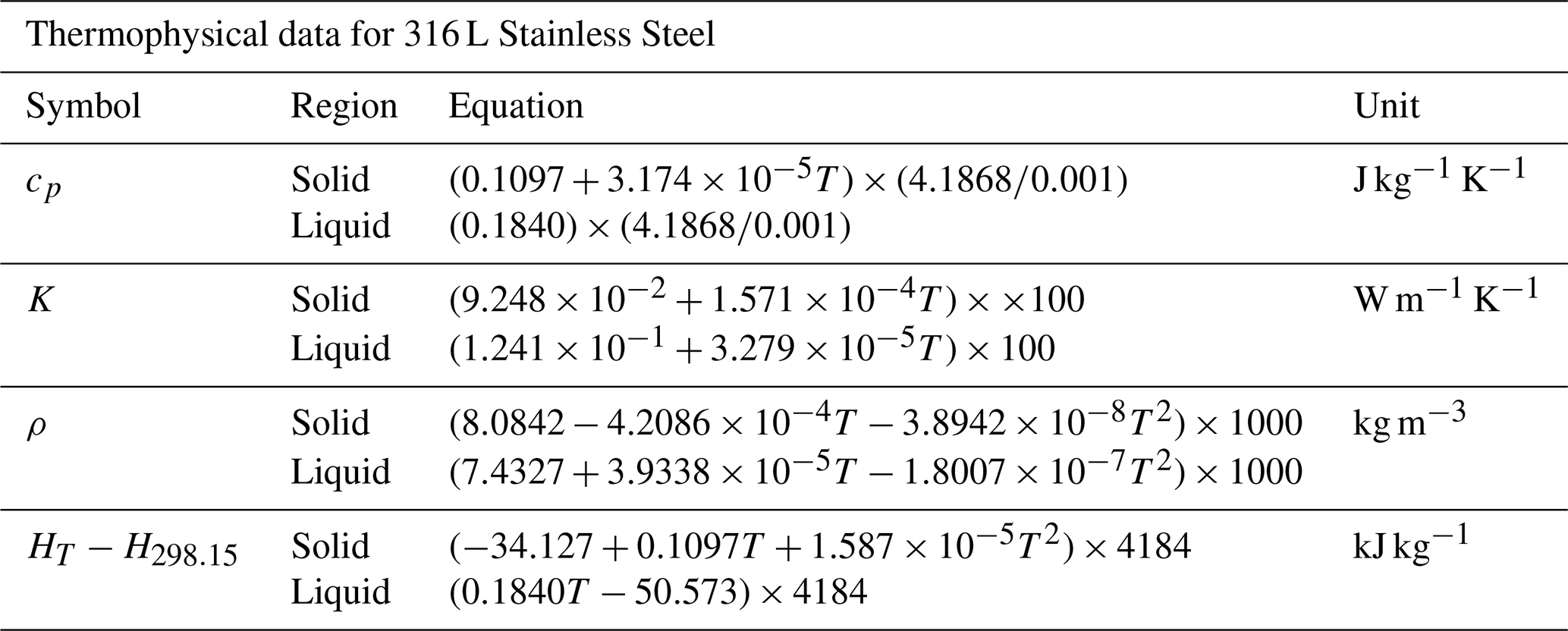
Temperature-dependent thermophysical data for 316 L stainless steel (Kim, 1975) has been considered. Table 2 shows the physical process parameters of the material adopted to simulate the process. Table 3 shows the variation of material properties such as heat capacity at constant pressure cp, thermal conductivity K, density ρ, specific enthalpy HT−H298.15.

Table 3Thermophysical data for the solid and liquid region of 316 L stainless steel.
2.4 Meshing and mesh refinement
The geometry of the cylindrical rod has been discretised in each of the modelling cases. For the FVM model, the size of the control volume Δx (Fig. 2) is considered as a discretisation parameter along with the time step Δt. Values of Δx was selected at 0.043, 0.0375 and 0.033 mm. In order to fulfil the stability condition, the value of Δt was varied from 0.00026 to 0.00016 s. In the final analysis, stable values of temperature distribution were obtained for Δx and Δt of 0.033 mm and 0.00016 s respectively.
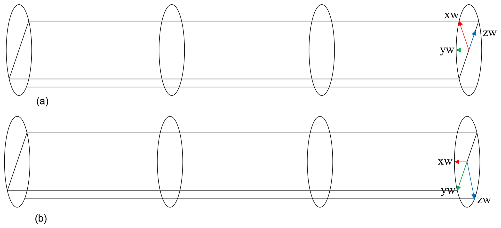

Figure 6Mesh refinement study using COMSOL Multiphysics® and mesh element sizes used for Combination-6.
As discussed for the FEM model, the length of the rod is segmented equally by 50 mm with each segment being discretised with various combinations of mesh size from coarser to finer. The qualitative descriptions coarse, fine, and finer are proprietary terms used in COMSOL Multiphysics®. In order to prevent asymmetry in the results, two work planes were introduced on the XZ (Fig. 5a) and ZY (Fig. 5b) planes along with partition domains. This forced the mesh to place a node in the centre of the cylindrical rod, allowing for the mesh to be symmetric.
A free tetrahedral element type was used in the FEM model. Consequently, each segment of the rod was meshed with elements ranging from a coarse mesh having 2478 elements to the finest mesh having 35 340 elements. Figure 6 shows examples of the meshed geometry of the rod with six different combination of elements used in the refinement study.
It was observed that the temperature distribution did not change significantly between combination 5 and 6 meshed rods. Combination-6 was selected for segment-1, the corresponding mesh element sizes used can be found in Fig. 6.
The data extracted after convergence and mesh independency tests has been used to plot and compare the simulation results obtained by each thermal model.

Figure 7Comparison of thermal histories obtained by the non-commercial and commercial model.
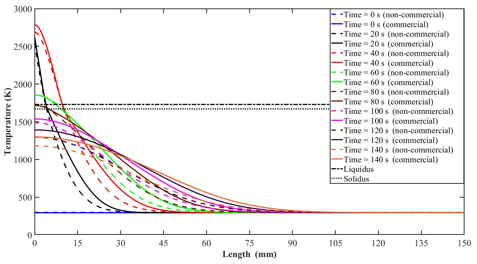
Figure 8Comparison of temperature distribution obtained by the non-commercial and commercial model along the length of the cylindrical rod.
Figure 7 shows the comparison of the thermal histories obtained from each model. The time versus temperature thermal histories were plotted for different locations along the length of the cylindrical rod. The liquidus and solidus temperatures are indicated for reference purposes.
Figure 8 demonstrates the temperature distribution along the length of the cylindrical rod for each model. The temperature profiles are shown at time intervals of 20 s.
Following on from the temperature profiles, Fig. 9 provides the comparison of the peak temperatures observed along the length of the rod throughout the entire simulation.
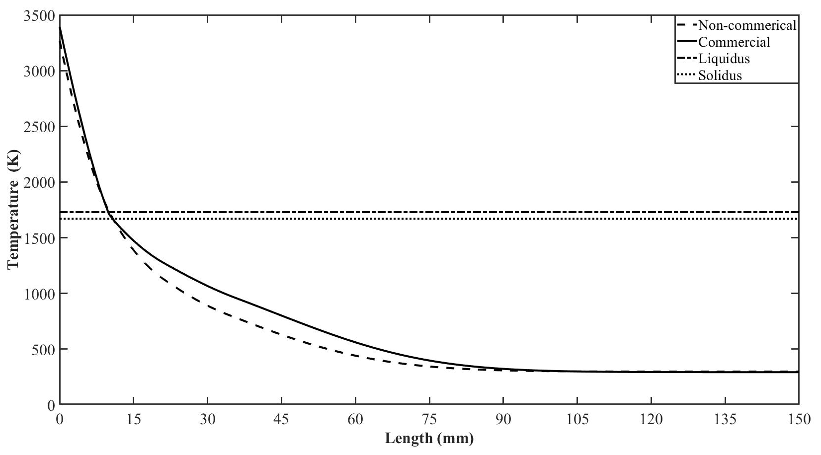
Figure 9Comparison of maximum value of temperature obtained by the non-commercial model and commercial model along the length of the cylindrical rod.
Figure 10 shows the simulated value for the melt pool depth obtained using both non-commercial and commercial models. The melt pool depth was defined by the axial position of the liquidus isotherm, i.e., 1730 K.
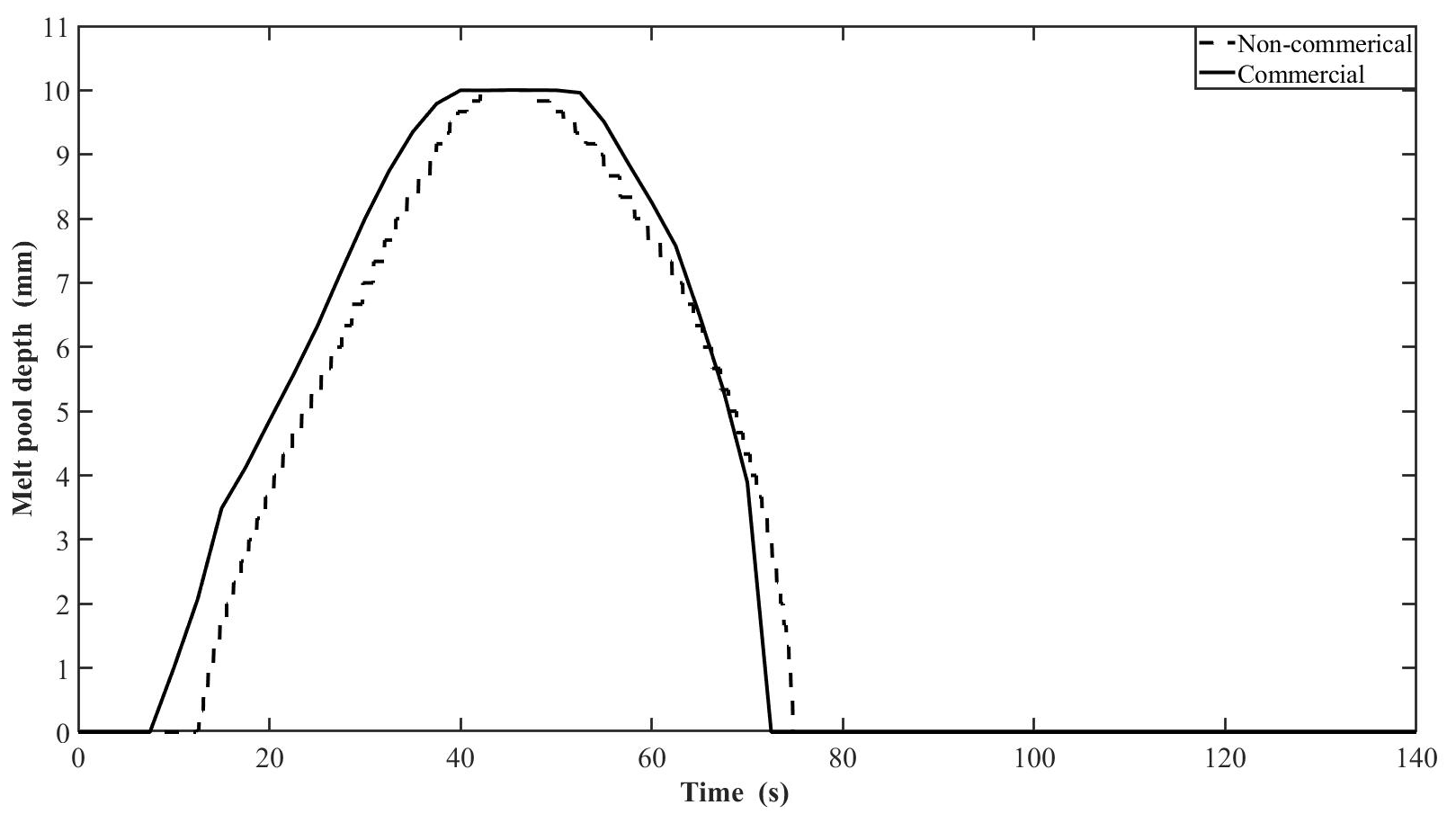
Figure 10Comparison of melt pool depth obtained by non-commercial and commercial model along the length of the cylindrical rod.
Figure 11 provides greater detail from the 3D FEM model. Figure 11a shows the variation in the temperature distribution captured over 20 s time intervals. Figure 11b depicts the lengths of the melt pools in segment-1 captured over 20 s time intervals. This figure distinguishes the existence of various phases in segment-1. In Fig. 11b it is possible to distinguish the mushy zone between 1670 and 1730 K.
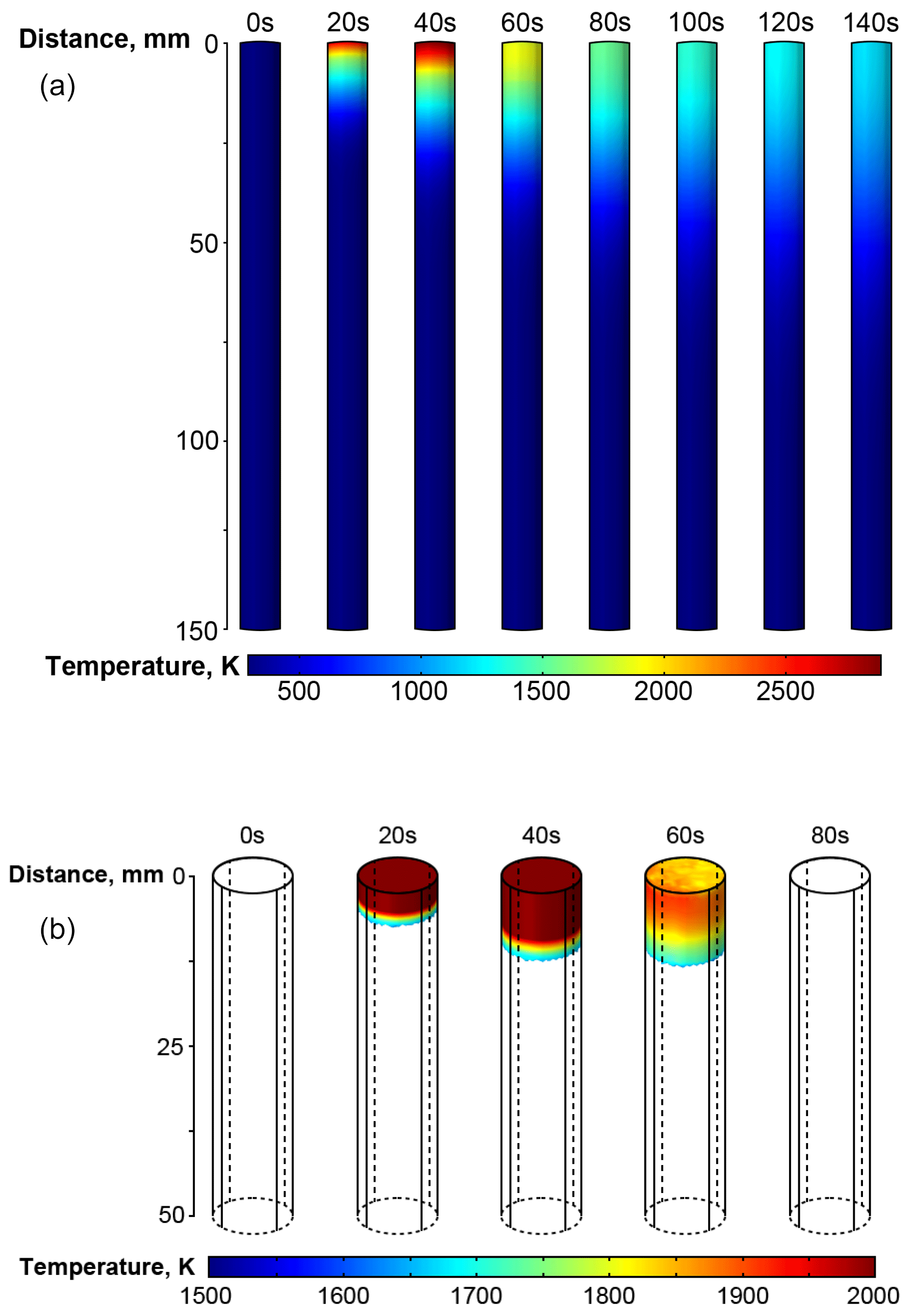
Figure 11(a) Temperature distribution along the length of the cylindrical rod. (b) The melt pool depth in segment-1.
4.1 Comparison of thermal histories
Figure 7 shows thermal histories at different locations for each model. The comparison shows qualitative agreement between the codes. However, the results show under prediction from the non-commercial model compared with results from the commercial model. For example, the times required for each model to reach the liquidus temperature (1730 K) at the nearest boundary are 11.5 and 8.5 s for the non-commercial and commercial model, respectively. On cooling from above the liquidus, the effect of latent heat is clear in the results for each model.
4.2 Comparison of temperature distributions along the length of the cylindrical rod
Comparing the temperature distribution (as shown in Fig. 8) recorded along the length of the cylindrical rod every 20 s revealed the heat transfer phenomenon within the cylindrical rod. At 40 s, the extent of the liquid and mushy zones (as given by the positions of the liquidus and solidus isotherms) predicted by the non-commercial model is 9.7 and 10.35 mm. Whilst the corresponding positions of the liquid and mushy zones predicted by the commercial model are 9.6 and 10.21 mm.
4.3 Comparison of maximum temperatures along the length of the cylindrical rod
Figure 9 compares the maximum temperature at each location along the cylindrical rod over all times. This data demonstrates a good agreement between both the non-commercial and commercial model. It was observed that the non-commercial model predicted the maximum temperature within a percentage difference of 4 % when compared to the commercial model.
4.4 Comparison of the melt pool depth
Figure 10 shows the prediction of the melt pool depth as characterised by the liquidus isotherm positions obtained for each model. The maximum melt pool depth predicted by each model were almost coincident at approximately 10 mm.
4.5 Temperature distribution
Figure 11 presents temperature distribution within the melt pool obtained by the commercial model. It shows the axial heat transfer along the length of the cylindrical rod (Fig. 11a) and the extent of the melt pool (Fig. 11b). It can be observed from Fig. 11 that the cylindrical rod experiences a continuous heating and cooling cycle from 0 to 140 s. For 20 to 40 s time interval, the melt pool depth gradually expands along the length of the cylindrical rod in agreement with Fig. 8.
This paper describes the development of two modelling applications and their code-to-code verification. Referring to the original aims and objectives the following conclusions can be drawn from the present work:
-
A non-commercial code for heat transfer simulation using a bespoke MATLAB® (FVM) approach and a commercial thermal model using COMSOL Multiphysics® (FEM) were developed with each model having the ability to simulate heat transfer within a cylindrical rod using a point heat source at the near boundary.
-
Mesh independency tests revealed that the results obtained from the non-commercial and commercial models were mesh independent allowing for meaningful and appropriate model verification.
-
Thermal histories, temperature distributions, maximum temperatures and melt pool depths across the sample have been investigated. Good qualitative agreement has been achieved by the non-commercial and commercial models. Temperature distribution along the length of the cylindrical rod allowed for the quantification of the dimensions of the liquid and mushy zones with each model producing similar outputs. It was observed that the non-commercial model predicted the maximum temperature within a percentage difference of 4 % as compared to commercial model. The melt pool depth predicted by both models were nearly coincident with each other.
-
The commercial model was used to predict the temperature distribution within the cylindrical rod, whilst visualising the details of the axial transfer along the length of the cylindrical rod. The model has the ability to demonstrate the depth at which the heat is transferred along the length of the rod as the power follows a transient profile.
The verification exercise presented in this manuscript is classified as an assurance step for future development of the current 3D FEM model. Imminent work on the present model will involve a moving point heat source and layer addition with the potential of application to both welding and metal additive manufacturing processes.
Contact the corresponding authors for code availability.
AMVH and SM were responsible for conceptualisation. AMVH, SM and SHN developed the relevant models and are accountable for data curation, formal analysis and methodology. AMVH and SHN completed the verification study. HW contributed to manuscript preparation and graphical visualisation. All authors contributed to the writing and reviewing of the document. SM and JQ were responsible for the project administration and supervision of this verification exercise. AMVH was responsible for the final compilation of this manuscript.
The authors declare that they have no conflict of interest.
The views and opinions in this document do not necessarily reflect those of the European Commission or the Special EU Programmes Body (SEUPB).
The North West Centre for Advanced Manufacturing (NW CAM) project is supported by the European Union's INTERREG VA Programme, managed by the Special EU Programmes Body (SEUPB).
If you would like further information about NW CAM please contact the lead partner, Catalyst, for details.
This research has been supported by the INTERREGVA (Project ID: IVA5055, Project Reference Number: 047).
This paper was edited by Daniel Condurache and reviewed by Deepak Kumar and one anonymous referee.
Battaglioli, S., Robinson, A. J., and McFadden, S.: Axisymmetric front tracking model for the investigation of grain structure evolution during directional solidification, Int. J. Heat Mass Tran., 115, 592–605, https://doi.org/10.1016/j.ijheatmasstransfer.2017.07.095, 2017a.
Battaglioli, S., McFadden, S., and Robinson, A. J.: Numerical simulation of Bridgman solidification of binary alloys, Int. J. Heat Mass Tran., 104, 199–211, https://doi.org/10.1016/j.ijheatmasstransfer.2016.08.030, 2017b.
COMSOL Multiphysics® v. 5.4: Phase Change User's Guide, 1–18, https://doi.org/10.1007/978-1-4684-0412-8_12, 2018.
Kim, C. S.: Thermophysical properties of stainless steels, Argonne National Laboratory, Argonne, IL, USA, 1975.
McFadden, S., Mooney, R. P., Sturz, L., and Zimmermann, G.: A Nucleation Progenitor Function approach to polycrystalline equiaxed solidification modelling with application to a microgravity transparent alloy experiment observed in-situ, Acta Mater., 148, 289–299, https://doi.org/10.1016/j.actamat.2018.02.012, 2018.
Mooney, R. P. and McFadden, S.: Order verification of a Bridgman furnace front tracking model in steady state, Simul. Model. Pract. Th., 48, 24–34, https://doi.org/10.1016/j.simpat.2014.07.005, 2014.
Mooney, R. P., McFadden, S., Rebow, M., and Browne, D. J.: A front tracking model for transient solidification of Al-7wt%Si in a Bridgman furnace, Trans. Indian Inst. Met., 65, 527–530, https://doi.org/10.1007/s12666-012-0201-2, 2012.
Mooney, R. P., Sturz, L., Zimmermann, G., and McFadden, S.: Thermal characterisation with modelling for a microgravity experiment into polycrystalline equiaxed dendritic solidification with in-situ observation, Int. J. Therm. Sci., 125, 283–292, https://doi.org/10.1016/j.ijthermalsci.2017.11.032, 2018.
Naumann, R. J.: An analytical approach to thermal modeling of bridgman-type crystal growth. II. Two-dimensional analysis, J. Cryst. Growth, 58, 569–584, https://doi.org/10.1016/0022-0248(82)90144-0, 1982.
Pelletier, D. and Roache, P. J.: Verification and Validation of Computational Heat Transfer, in: Handbook of Numerical Heat Transfer: Second Edition, edited by: Minkowycz, W. J., Sparrow, E. M., and Murty, J. Y., 417–442, John Wiley & Sons, Hoboken, New Jersey, USA, 2000.
Pineau, A., Guillemot, G., Tourret, D., Karma, A., and Gandin, C. A.: Growth competition between columnar dendritic grains – Cellular automaton versus phase field modeling, Acta Mater., 155, 286–301, https://doi.org/10.1016/j.actamat.2018.05.032, 2018.
Roache, P. J.: Verification and Validation in Computational Science and Engineering, in Computing in Science Engineering, 107–240, Hermosa, available at: https://pdfs.semanticscholar.org/0f3c/728bd0f17e45cce72bda2165707a0eb9e03b.pdf (last access: 29 October 2019), 1998.
Roache, P. J.: Verification of codes and calculations, AIAA J., 36, 696–702, https://doi.org/10.2514/3.13882, 2012.
Seredynski, M., Battaglioli, S., Mooney, R. P., Robinson, A. J., Banaszek, J., and McFadden, S.: Code-to-code verification of an axisymmetric model of the Bridgman solidification process for alloys, Int. J. Numer. Method. H., 27, 1142–1157, https://doi.org/10.1108/HFF-03-2016-0123, 2017.