the Creative Commons Attribution 4.0 License.
the Creative Commons Attribution 4.0 License.
 | 10 Jan 2019
Solution-region-based synthesis approach for selecting optimal four-bar linkages with the Ball–Burmester point
Lairong Yin
Long Huang
Juan Huang
Lei Tian
Fangyi Li
In this paper, we present a solution-region-based synthesis approach for selecting optimal four-bar linkages with a Ball–Burmester point. We discuss both general and special cases of the Burmester point that coincide with the Ball point at the pole of the inflection circle. Given the coordinates of one fixed joint, any point on the target's straight line, and the direction of this straight line, we can synthesize an infinite number of mechanisms using a coupler curve with five-point contacts with its tangent by adopting the proposed approach. Each initial parameter corresponds to three side links that can generate three four-bar mechanisms. We generate different mechanism property charts by developing mechanism software that enables users to intuitively identify relevant linkage information and select the optimal linkage. This novel approach is a visualized analytical method for synthesizing and selecting optimal four-bar linkages with one Ball–Burmester point on its coupler curve.


As an important planar four-bar mechanism, four-bar linkages that approximate a straight line have been widely studied based on the theory of the kinematic geometry of mechanisms (Dijksman, 1976; Hunt, 1987; McCarthy, 2000; Wang and Wang, 2015). Dijksman (1972) and Dijksman and Smails (2000) used a geometrical method to discuss the Ball point in different configurations. Tesar et al. (1967) and Vidosic and Tesar (1967a, b) derived a series of synthesis formulas, and transformed the results into design diagrams for users according to three different cases, i.e., the general case of the Ball–Burmester point, the special case of the Ball–Burmester point at the inflection pole, and the special case of the Ball-Double Burmester point. Yu et al. (2013) presented a numerical comparison synthesis method for single and double straight-line guidance mechanisms to solve four-bar straight-line guidance mechanism synthesis problems for an arbitrarily given straight line's “angle requirement” and “point-position requirement”. Han (1993) studied the synthesis of the four-bar straight-line linkage of Ball and Burmester points in general cases. The author Yin et al. (2011, 2012) studied the synthesis of the straight-line linkage of Ball and Burmester points, separately. Han et al. (2009) proposed a solution-region-based method for linkage synthesis to obtain the optimal solution in the feasible solution region, and extended their approach to four-position finitely separated and mixed “point-order” positions (Yang et al., 2011), six-bar motion generation (Cui and Han, 2016), and RCCC Linkages (Han and Cao, 2018; Bai and Angeles, 2015). Traditional synthesis methods use congruence to represent infinite parametric solutions. The solution-region method is an optimal-mechanism synthesis approach for expressing infinite solutions on finite diagrams for cases irrespective of whether the congruence method can be used. Bai and Angeles (2015) proposed a new method for calculating cognate mechanisms, and cognate straight-line mechanisms can be obtained by employing this approach. However, none of the above authors have made a systemic study of how to choose desired straight-line mechanisms with a Ball–Burmester point from an infinite number of synthesized mechanisms, and that satisfy the target constraints.
Here, we present a visualized synthesis approach based on the solution region for selecting optimal four-bar linkages with a Ball–Burmester point. We discuss both the general and special cases of the Burmester point that coincide with the Ball point at the pole of the inflection circle. Different mechanism property charts are generated by developing mechanism software to enable users to intuitively identify information about the involved linkages and to select the optimal linkage from an infinite number of mechanism solutions.
Robert Ball proposed the famous Ball point theory, which is based on the infinitesimal displacement and instantaneous invariance of curvature. The Ball point is defined as the point whose radius of curvature is infinite and whose curvature is stationary, which is the intersection point of the inflection circle and the cubic of stationary curvature at a certain instant (other than the polar point P). The linkage curve and its tangent line have an osculation of no less than three orders on the Ball point, which means it passes through four points that are infinitely close to each other. The velocity, acceleration, and jerk of the Ball point in a moving rigid body have the same direction. Four-bar linkages that approximate a straight line with four contacting points can be synthesized using the Ball point.
The Burmester point is a higher-order stationary point of the cubic of a stationary curvature, whose trajectory intersects with the curve at no less than five infinitely close points, namely a four-order osculating. In this paper, we used the theory of the Burmester point to develop a method for synthesizing a five-point contact mechanism that approximates a straight line under both general and special conditions. The proposed method allows the designer to give a fixed hinge point, the points on the straight line, and the direction of the line.
2.1 General case
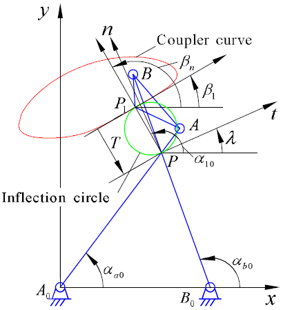
Assume a fixed joint point and a point on a straight line, where the direction of the straight line is β1 and the displacement is T. Vector T (T≠0) points from the Ball point P1 to the polar point T. We note that the parameter λ at point P between the t axis and x axis is known during the synthesis of the five-point contact mechanism that approximates a straight line, as compared with the case of four-point contact (Yin et al., 2012). Parameters αa0,αb0, αb0, αc0, and α10 are defined as the angles from the positive direction of the T axis to the vectors B, B0P, C0P, and PP1, respectively. Vectors αa0,αb0, αb, αc, and α10 are defined as , , , and , respectively. For simplicity of calculation, let diameter D of the inflection point circle be 1. The expected mechanism can be obtained by scaling the synthesized mechanism by the diameter of the inflection point circle. Furthermore, the coordinates of another fixed joint B0 and two motion joints A and B must be determined to synthesize four-bar mechanisms that approximate a straight line. Details regarding the definition of parameters are taken from Figs. 1 and 2 in reference of Yin et al. (2012), as shown in Fig. 1.
According to the kinematic geometric theory of infinitely close positions, several points can be selected from a motion plane at any instantaneous position, whose trajectory has fourth-order contact with its curvature circle. This means that these points are the circle points of five infinitely close positions, namely Burmester points, which are higher-order stationary points of the trajectory curvature. Using the Euler-Savary equation (Yin et al., 2012) to solve the two-order derivative equation , or using the curvature stagnation point curve equation to obtain the first derivative equation , we obtain:
where N and M are two auxiliary variables defined as follows:
Equation (1) is a quartic equation that has four real roots at most. These four roots have the value αi of the polar coordinates of the Burmester point. Motion joints A and B correspond to roots αa and αb, respectively, and the connecting rod point P1 corresponds to root α1. We assume the other motion joint is C, which corresponds to root αc.
After we determine the instantaneous center P and parameter λ, by definition, we can obtain angles α1 and αa directly. αb and αc are solved as follows.
According the relation between the fourth-order equation root and coefficient of Eq. (1), we obtain:
or
Assuming tanα1 in Eq. (4) and tanαc in Eq. (5) are the two roots of a quadratic equation, and according to the Vieta theorem, we have the following:
Similarly, Eq. (6) can be regarded as the quadratic equation of tanα, and according to the Vieta theorem, the roots of Eq. (6) are imaginary when:
Therefore, the other two Burmester points are imaginary. Combining Eq. (6) with the cubics of stationary curvature equations, we have the following:
By substituting PP1=Dsinα1 into Eq. (10), and assuming D equals 1, we obtain:
By substituting Eq. (11) into Eq. (6) and doing some rearranging, we have the following:
where U=tanαatanαb and . By substituting Eq. (12) into Eq. (11) and doing some rearranging, we obtain:
Furthermore, by substituting Eqs. (11) and (13) into the Euler–Savary equation: ,
we obtain the following:
Since the diameter D of the inflection-point circle equals 1, by combining it with Eq. (14), we obtain:
By substituting Eq. (16) into Eq. (4) and doing some rearranging, we have:
Considering that motion joints C and B are Burmester points, we replace joint B in Eq. (15) with joint C and substitute Eq. (17) into Eq. (15). Then, PC can be obtained similarly, as follows:
According to the Euler-Savary equation:
By substituting Eq. (21) into Eq. (14), we obtain:
Equation (22) can be regarded as an equation for the unknown αb. After rearranging, we have:
where: ; ; G=PAtanαatanα1sinαa.
There are two roots for αb in Eq. (23), which are assumed to be αb1 and αb2. So, we have:
PB can be obtained by substituting αb into Eq. (15), and furthermore, PB0 can be calculated using Eq. (20). We note that there is no real root for αb when .
The values of PC and PC0 can be determined similarly, and the diameter of the actual inflexion circle can be calculated using the equation PP1=Dsinα1. After calculating PA, PA0, PB, PB0, PC, and PC0, we can obtain the actual size of the mechanism by multiplying these values by the actual diameter of the inflection point circle.
The coordinates of motion joints A, B, and C and fixed joints C0 and B0 can be calculated as follows:
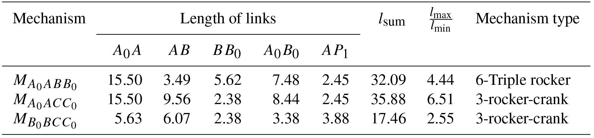
For a given set of conditions including a fixed joint A0, a point P1 on a straight line, the direction of the straight line β1, displacement T, and parameters λ, we can calculate three sets of connecting rods AA0, BB0, and CC0 using the proposed method. By arbitrarily selecting two connecting rods from AA0, BB0, and CC0, we obtain a four-bar linkage that approximates a straight line. Since αb has two roots αb1 and αb2, a set of given conditions corresponds to six five-point-contact four-bar linkages that approximate a straight line. However, the fact that connecting rod BB0 corresponds to αb1 is the same as connecting rod CC0 corresponding to αb2. Also, the fact that connecting rod CC0 corresponds to αb1 is the same as connecting rod BB0 corresponding to αb2. Therefore, there are only three four-bar linkages.
2.2 Special condition: Burmester point located at the pole of the inflection circle
When the Burmester point is located at the pole of the inflection circle, parameter λ cannot be determined arbitrarily. Below, we calculate the coordinates of another fixed joint B0 and two motion joints A and B.
When the Burmester point coincides with the Ball point at the pole of the inflection circle, α1 equals 90∘. The coordinates of the instantaneous center P can be determined by its definition. According to the definition of parameter λ, we have:
By substituting into Eq. (14), and assuming that tanα1 approaches positive infinity, we have:
where U=tanαatanαb and . Another Burmester point can be obtained using Eqs. (17) and (18). Using Eq. (4), we have:
By substituting Eq. (34) into the equation for the curvature of a point on the curve, we obtain:
We can then derive PA, PA0, and PB0 from the formula in reference (Yin et al., 2011). The coordinates of joints A, B, and B0 can be calculated using Eqs. (26), (27), and (28), respectively, and the coordinates of joints C and C0 are as follows:
Unlike the general condition, when the Burmester point coincides with the Ball point at the pole of the inflection circle, αb has only one root. Therefore only three five-point-contact four-bar linkages that approximate a straight line can be obtained with a given set of conditions.
3.1 General case
3.1.1 Solution-region generation
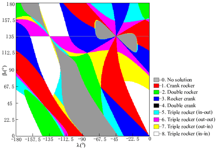
According to the given conditions, the solution region of the mechanism is analyzed on the coordinate plane β1-λ. Since αb may have no real root, if direction β1, displacement T, and angle λ are given arbitrarily, some solution regions will have no mechanism solution, and these are infeasible mechanism regions. Because there are three variables (β1, T, and λ), a square solution region can be obtained for any pairs of these three variables. Therefore, there will be three solution region diagrams according to the three variables (β1, T, and λ).
3.1.2 Example
The task is to design four-bar linkages that approximate a straight line with the following conditions: fixed joint , a point on the straight line, and the displacement T=5. Also, the synthesized four-bar linkages should be five-point-contact linkages that approximate a straight line.
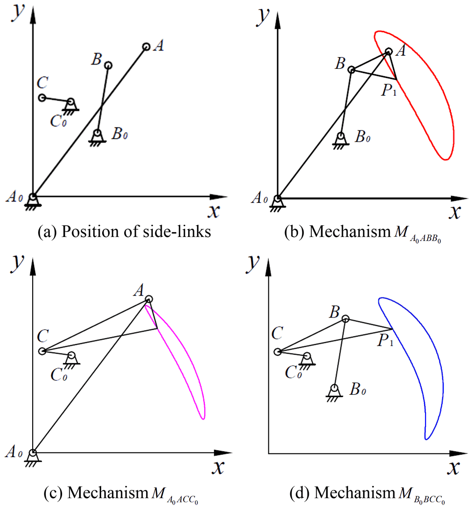
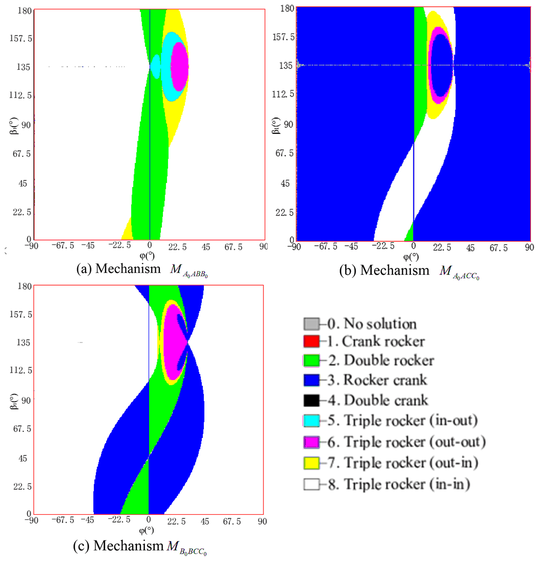
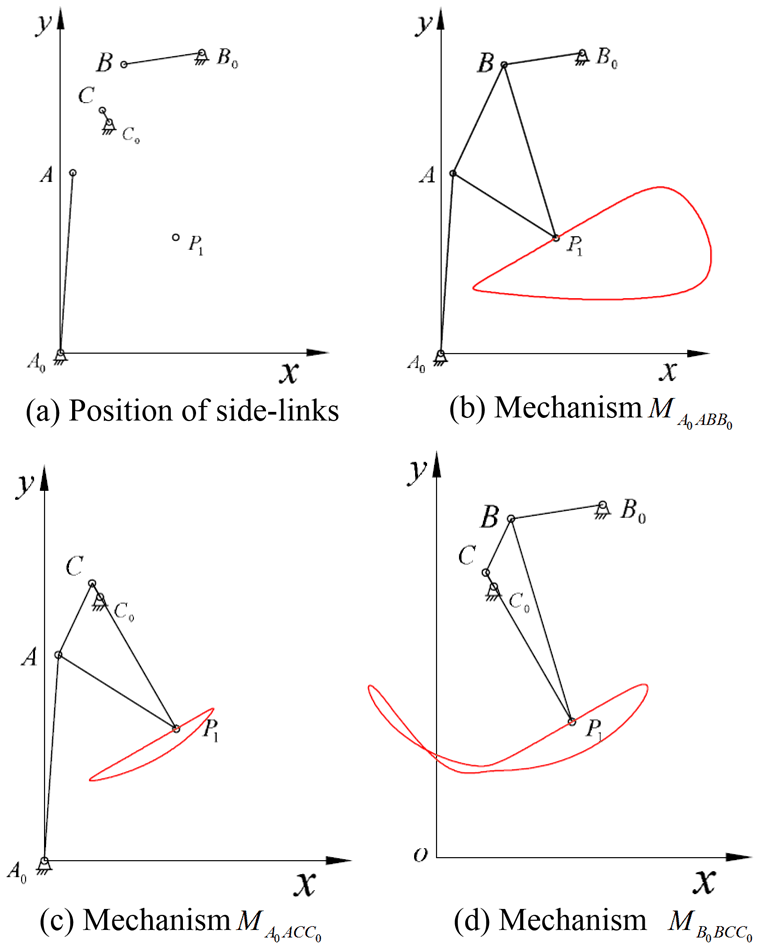
There are three solution-region diagrams. In the mechanism-type solution region diagram of mechanism shown in Fig. 2, we assume that direction β1 equals 120∘ and angle λ equals −85∘, and then we have three synthesized linkages that approximate a straight line, as shown in Fig. 3d, the parameters of which are shown in Table 1. The other two synthesized mechanisms and are shown in Fig. 3b and c. The classification of planar four-bar linkages is performed with reference to the method developed by Barker (1985):
- 0.
No solution,
- 1.
Crank rocker,
- 2.
Double rocker,
- 3.
Rocker crank,
- 4.
Double crank,
- 5.
Triple rocker (in–out),
- 6.
Triple rocker (out–out),
- 7.
Triple rocker (out-in), and
- 8.
Triple rocker (in-in).
3.2 Special condition: Burmester point located at the pole of the inflection circle
3.2.1 Solution-region generation
If T varies from −∞ to +∞ continuously and β1 is determined arbitrarily, then the infinite mechanisms can be obtained. Similarly, if β1 varies from 0 to 180∘ continuously and T is determined arbitrarily, then the infinite mechanisms can be obtained. All the above mechanism solutions constitute the solution region. In the solution region, the area that satisfies the design requirements is the feasible solution region.
To illustrate all the mechanism solutions in the finite coordinate plane, displacement is expressed as the parametric equation of angle , as follows:
where k1 is the step-size factor, which is used to adjust the mechanism solution region to show the required mechanism solution region.
When T is infinite, and we use the above general synthetic equations to solve the mechanism, the resultant mechanism has some poor quality properties, i.e., the length ratio of the mechanism and the relative linear length. To improve these properties, we can use the synthesis formula for four-bar linkages that approximate a straight line with an infinite instant center, which we do not discuss here.
If we let k1=24, the square diagram of the mechanism solution region is as shown in Fig. 4.
3.2.2 Example
In this task, we design four-bar linkages that approximate a straight line and which satisfy the following conditions and requirements: Given a fixed joint and a point on the straight line, the Burmester point of the resultant mechanism should be the pole of the inflection circle.
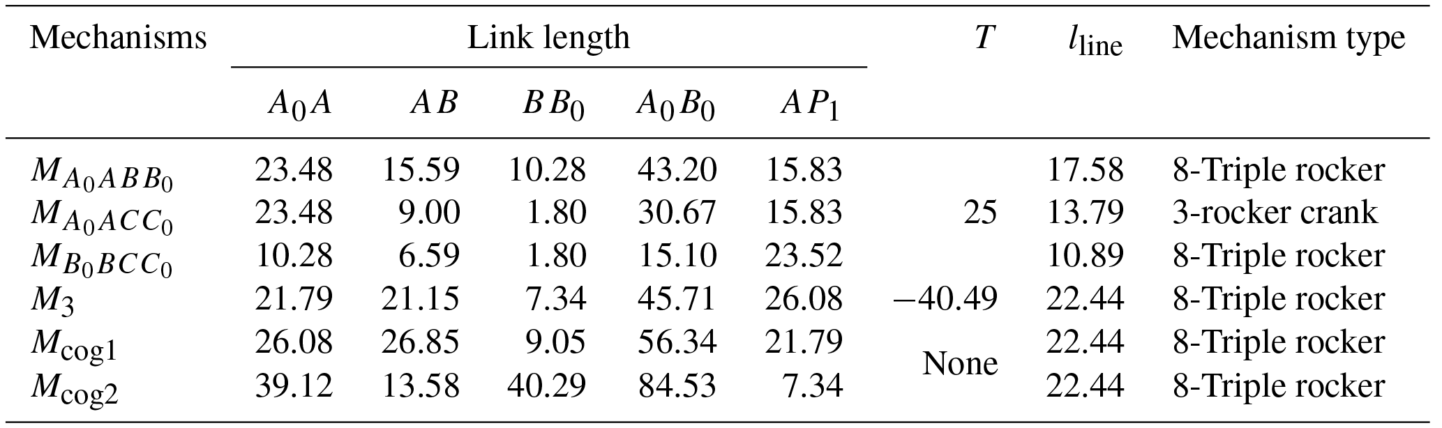
Let β1 be 30∘ and let T be 25. The three resultant mechanisms are shown in Fig. 5, and their parameters are shown in Table 2.
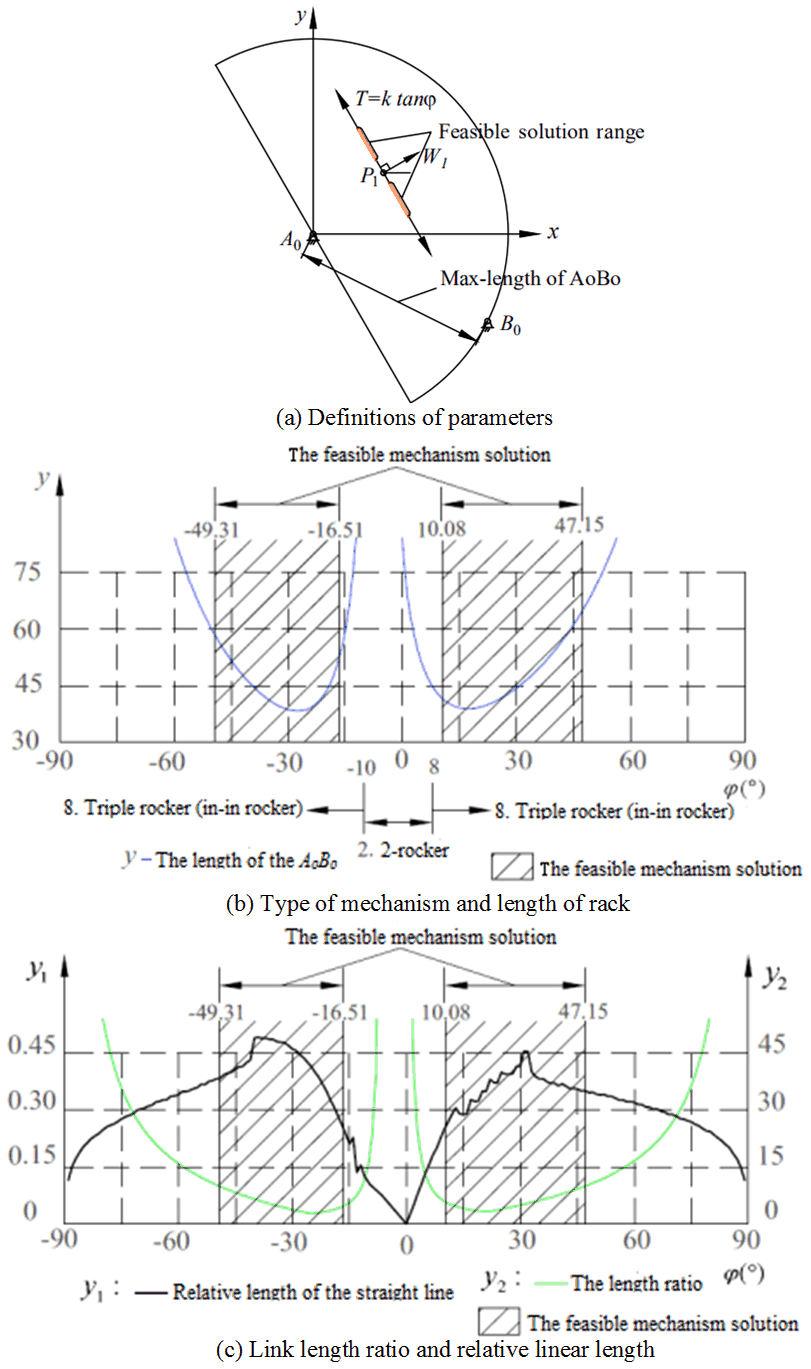
To synthesize the optimal mechanism solutions when the direction of the straight line is 30∘, we use the proposed synthesis software to plot the mechanism solution region curves, which utilizes a method similar to that used for the circular mechanism solution regions. Take mechanism A0ABB0 for instance. The design constraints are as follows: the frame length A0B0 is less than 70, the link length ratio is less than 10, and the relative length of the straight line is longer than 0.25.
Let k1 be 50, which means T=50tanφ. When T varies continuously, the performance curves of the resultant mechanisms are as shown in Fig. 6. The y-coordinates represent the length of the frame A0B0, the relative length of the straight line, and the length ratio of the links. The shaded area is the feasible mechanism solution area that satisfies the design constraints, as shown above the x-coordinates. The mechanism-type distributions are shown below the x-coordinates.
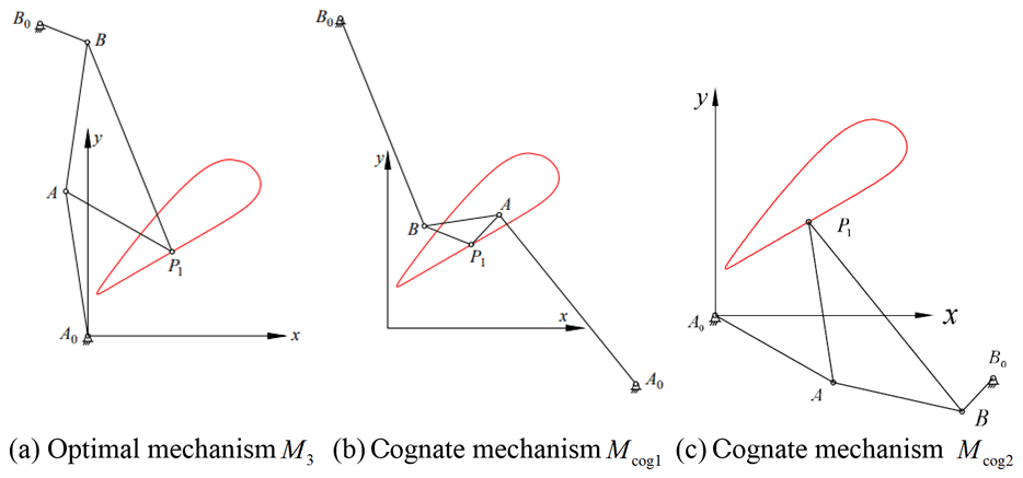
Figure 6c shows that the relative length of the straight line is longest when φ equals −39∘, and that the length ratio and the length of the frame are within the design constraints. The corresponding mechanism is shown in Fig. 7a, and its parameters are shown in Table 2. Note that the physical length of the straight line can be obtained by multiplying the relative length of the straight line by the frame length. The other two cognate mechanisms for the straight-line linkage in Fig. 7a, based on the Roberts–Chebyshev Theorem, are shown in Fig. 7b and c.
In this paper, to select optimal four-bar straight-line linkages, we discussed both the general and special cases of the Burmester point that coincide with the Ball point at the pole of the inflection circle. By adopting our proposed approach, an infinite number of mechanisms with a coupler curve that has five-point contacts with its tangent were obtained. We generated different mechanism property charts by developing a mechanism software to enable users to intuitively identify information about the involved linkages and to select the one that is optimal. The results of the calculation examples indicated that the proposed method works effectively. This is a novel visualized analytical method for synthesizing and selecting optimal four-bar linkages with one Ball–Burmester point on its coupler curve.
Using the proposed method, we found there to be three straight-line linkages with the same straight-line segment of a coupler curve for each of the initial parameters given. However, the coupler curves of three cognate mechanisms by the Roberts–Chebyshev Theorem are identical. Therefore, after the initial parameters are given, we can synthesize three different mechanisms with the same straight-line segments of coupler curves by the proposed method. In addition, we can obtain the other two cognate mechanisms for each straight-line linkage based on the Roberts-Chebyshev Theorem.
All the data used in this manuscript can be obtained on request from the corresponding author.
LY proposed the idea and methodology; LH derived the equations; JH, LT and FL developed the software.
The authors declare that they have no conflict of interest.
This work has been financially supported by the National Natural Science
Foundation of China (No. 51705034-51805047), the Natural Science Foundation
of Hunan province (No. 2018JJ3548), and Innovation Platform Foundation of
Key Laboratory of Safety Design and Reliability Technology for Engineering
Vehicle of Hunan Provincial Department of Education (17K003).
Edited by: Chin-Hsing Kuo
Reviewed by: two anonymous referees
Bai, A. and Angeles, J.: Coupler-curve synthesis of four-bar linkages via a novel formulation, Mech. Mach. Theory, 94, 177–187, 2015.
Barker, C. Ā.: A complete classification of planar four-bar linkages, Mech. Mach. Theory, 20, 535–554, 1985.
Cui, G. Z. and Han, J. Y.: The solution region-based synthesis methodology for a 1-DOF eight-bar linkage, Mech. Mach. Theory, 98, 231–241, 2016.
Dijksman, E. A.: Approximate straight-line mechanisms though four-bar linkages, Romanian Journal of Technical Science, Applied Mechanics, 17, 319–372, 1972.
Dijksman, E. A.: Motion geometry of mechanisms, Cambridge University Press, 1976.
Dijksman, E. A. and Smails, A. T.: How to exchange centric inverted slider cranks with λ-formed 4-bar linkages, Mech. Mach. Theory, 35, 305–327, 2000.
Han, J. Y.: Ein Beitrag zur rechnerunterstuetzten Masssynthese ebener Gelenkgetriebe fuer angenaeherte Geradfuehrungen durch vier bzw. fuenf unendlich benachbarte Punkte, Dissertation Universitaet der Bundeswehr, 1993.
Han, J. Y. and Cao, Y.: Analytical synthesis methodology of RCCC linkages for the specified four poses, Mech. Mach. Theory, 133, 531–540, 2018.
Han, J. Y., Qian, W. X., and Zhao, H. S.: Study on synthesis method of λ-formed 4-bar linkages approximating a straight line, Mech. Mach. Theory, 44, 57–65, 2009.
Hunt, K. H.: Kinematic geometry of mechanisms, Clarendon Press, 1987.
McCarthy, J. M.: Geometric Design of Linkages, Springer-Verlag, 2000.
Tesar, D., Vidosic, J. P., and Wolford, J. C.: Selections of four-bar mechanisms having required approximate straight-line outputs, part II: the Ball–Burmester point at inflection pole, J. Mechanisms, 2, 45–60, 1967.
Vidosic, J. P. and Tesar, D.: Selections of four-bar mechanisms having required approximate straight-line outputs, part I: the general case of the Ball–Burmester point, J. Mechanisms, 2, 23–44, 1967a.
Vidosic, J. P. and Tesar, D.: Selections of four-bar mechanisms having required approximate straight-line outputs, part III, the Ball-Double Burmester point Linkage, J. Mechanisms., 2, 61–78, 1967b.
Wang, D. L. and Wang, W.: Differential geometry analysis and synthesis of mechanism motion, China Machine Press, 2015.
Yang, T., Han, J. Y., and Yin, L. R.: A unified synthesis method based on solution regions for four-position finitely separated and mixed “Point-Order” positions, Mech. Mach. Theory, 46, 1719–1731, 2011.
Yin, L. R., Han, J. Y., and Yang, T.: A synthesis and optimal method for straight line mechanism with Burmester point, 2nd International Conference on Manufacturing Science and Engineering, 199, 1240–1243, 2011.
Yin, L. R., Han, J. Y., and Mao, C.: Synthesis method based on solution regions for planar four-bar straight-line linkages, J. Mech. Sci. Technol., 26, 3159–3167, 2012.
Yu, H. Y., Zhao, Y. W., and Wang, Z. X.: Study on numerical comparison method of four-bar straight-line guidance mechanism, Journal of Harbin Institute of Technology, 20, 63–72, 2013.