the Creative Commons Attribution 4.0 License.
the Creative Commons Attribution 4.0 License.
 | 14 Jun 2019
Estimation of tool life and cutting burr in high speed milling of the compacted graphite iron by DE based adaptive neuro-fuzzy inference system
Longhua Xu
Chuanzhen Huang
Rui Su
Hongtao Zhu
Hanlian Liu
Yue Liu
Chengwu Li
Jun Wang
The studies of tool life and formation of cutting burrs in roughing machining field are core issues in high speed milling of compacted graphite iron (CGI). Changing any one of the cutting parameters like cutting speed or feed rate can result in varied tool life and different height of the cutting burrs. In this work in order to study the relationship between cutting parameters and tool life and height of the cutting burrs, a new differential evolution algorithm based on adaptive neuro fuzzy inference system (DE-ANFIS) as a multi-input and multi-output (MIMO) prediction model is introduced to estimate the tool life and height of the cutting burrs. In this model, the inputs are cutting speed, feed rate and exit angle, and the outputs are tool life and height of the cutting burrs. There are 12 fuzzy rules in DE-ANFIS architecture. Gaussian membership function is adopted during the training process of the DE-ANFIS. The proposed DE-ANFIS model has been compared with PSO-ANFIS, Artificial Neural Network (ANN) and Support Vector Machines (SVM) models. To construct the predictive models, 25 cutting data were obtained through the experiments. Compared with PSO-ANFIS, ANN and SVM models, the results indicate that DE-ANFIS can provide a better prediction accuracy of tool life and height of the cutting burrs, and achieve the required product and productivity. Finally, the analysis of variance (ANOVA) shows that the cutting speed and feed rate have the most effects on the tool life and height of cutting burrs, respectively.


The demand for high productivity and quality of heavy duty engines has been the driving force in the manufacturing field. Materials with better characteristics and performances than traditional grey iron are demanded for heavy duty engine. The compacted graphite iron (CGI), as one of the most important irons, plays an indispensable role in the machinery manufacturing industry. Compared with grey iron, CGI has a longer fatigue life (about twice as long), better tensile strength and a 40 % increase in elastic modulus. It is believed that CGI is the ideal metal for heavy duty engine material (Chuang et al., 2018; Varun et al., 2013; Qiu et al., 2018).
With the development of manufacturing technology, high speed machining (HSM) can have anywhere from 3–50 times higher efficiency than traditional machining. Relatively, CGI is a typically difficult-to-machine material, so studies of tool life become the focus of research in the rough machining CGI field. Ming et al. (2011) found that coated tools produce better surface quality and with better processing efficiency than non-coated tools in the milling process of CGI. Similarly, Gabaldo et al. (2010) studied the effect of cutting speed on the amount of material removed in milling of CGI. It turned out that with the cutting speed increased from 420 to 850 m min−1, tool life would decrease. In other work, Su et al. (2018) studied the effect of cutting parameters on the workpiece material removal volume in high speed milling of CGI. It was found that the tool life decrease, but the material removal volume increased when the cutting speed and feed rate increased. However, the estimation of tool life under multiple factors is still unclear for CGI.
As the CGI has outstanding ductility, the cutting burrs will appear on edges of the machined surface during the milling process of CGI. The cutting burrs formed on the workpiece can decrease the dimensional accuracy and surface integrity, meaning extra time would be expended to deburr. Hence, the economic benefit is reduced at the same time. Another factor to be considered is the implication of the exit angle. It is known that the cutting burr changes along the exit angle. Olvera and Barrow (1998) came to a conclusion that the exit angle and the tool nose geometry have a significant influence on the formation and characteristics of the burr that created on the exit edge. In other work, Chern (2006) found that as the exit angle increased from 0 to 180, different shapes of cutting burr appeared in milling, including knife-type and wave-type in face milling of alloys using cutter, and the exit angle also has a great influence on the height of the cutting burrs.
While more attention is focused on the nonlinear model, ANFIS model which combines neural network and fuzzy logic shows its advantages, because of its self-adaptive and high prediction accuracy ability. Mehmet et al. (2015) estimated the surface quality and cutting temperature in turning processes of noncorrosive steel using ANFIS with particle swarm optimization (PSO) learning. The results showed the predicting ability is 95.8 % for the surface quality and 97.4 % for cutting temperature. Gill et al. (2010) used ANFIS to establish the model of AISI M2 turning tools for estimating of the tool life, and the results showed the prediction agrees well with the testing data with the correlation coefficients of 0.99 and the mean absolute error of 2.4 %. In other work, Dong and Wang (2011) used ANFIS with leave one out-cross validation (LOO-CV) approach to predict the surface roughness in end milling process. Compared with the opponent methods, the prediction accuracy of ANFIS with LOO-CV approach can be improved to 96.4 %.
In recent years, group based heuristic search algorithm has attracted more and more attention which can be applied to solve machining problems. Differential evolution algorithm (DE) is an efficient global optimization algorithm. Yang et al. (2010) proposed DE based artificial neural network for the prediction of surface roughness in turning operations. The result shows that the convergence speed for the DE-based ANN is higher than the backpropagation-based ANN. Lee et al. (2016) proposed the Taguchi-sliding-based differential evolution algorithm (TSBDEA) to solve the problem of optimization for the surface grinding process. The results show the TSBDEA can be statistically sound and quickly convergent and obtain accurate results well for the surface grinding process. Wang et al. (2017) proposed the support vector machine and differential evolution for tool condition monitoring system. The results show that the classification accuracy of differential evolution-support vector machine is higher than the empirical selection-support vector machine.
It can be seen from the literature reviews above that lots of studies focus on predictions of the surface roughness of metallic materials. The studies seldom involve the predictions of tool life, especially for estimation of both tool life and cutting burr. Estimation of both tool life and cutting burr under different cutting parameters for CGI is quite important in process of high speed milling operations. In this work, a novel DE-ANFIS system is employed to effectively predict both tool life and height of the cutting burrs is proposed.
2.1 Equipment, cutting tool and workpiece materials
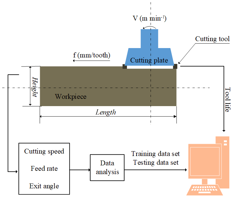
The high speed milling experiments without the aid of lubricating fluid have been carried out on a DAEWOO ACE-V500 South Korea) CNC machining center with speeds ranging from 80 to 10 000 rpm. The set-up of milling operation is shown in Fig. 1.
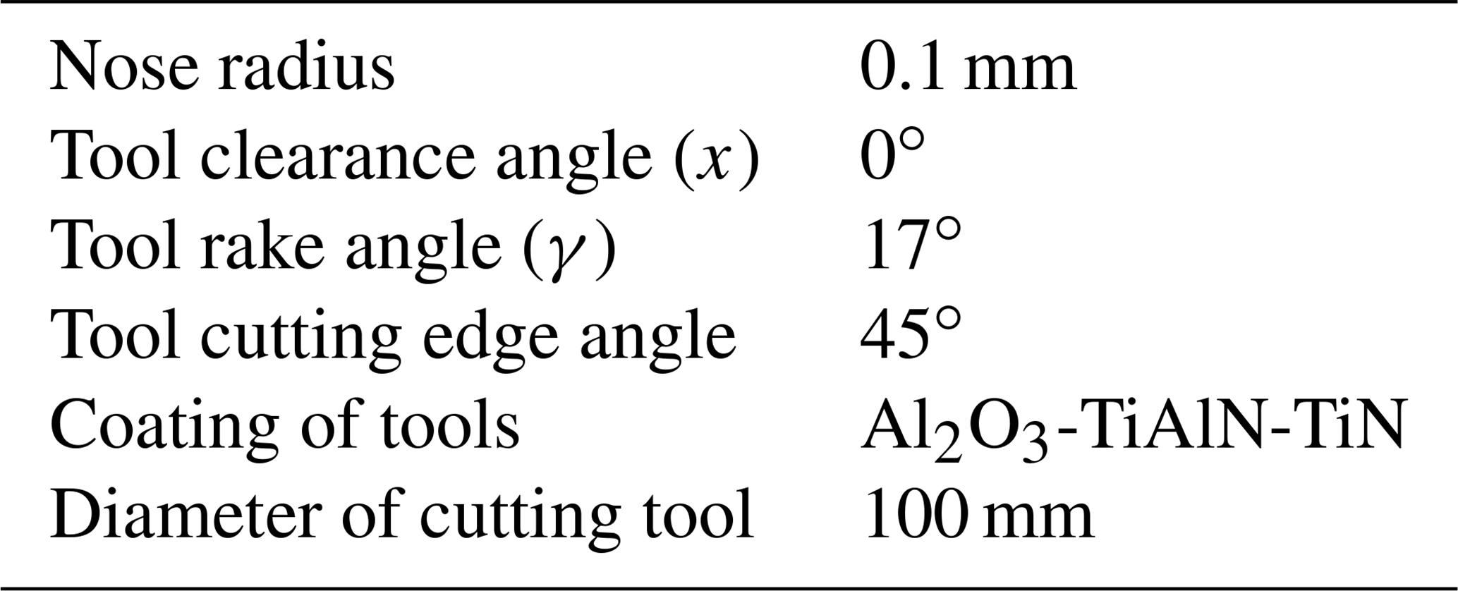
In the experiments, the grade of the workpiece material is GJV450 with pearlite main base structure, and the vermicular graphite rate is 90 %. The block size of workpiece is 200 mm (length) by 60 mm (width) by 80 mm (height). The adopted cutting tool is KENNMENTALHNGX090516-MR coated with , and the matrix material is cemented carbide substrate. Table 1 shows the detailed parameters of coated tool.
2.2 Measurement of tool life
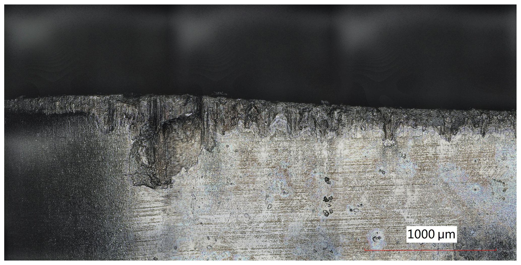
The face milling is an intermittent cutting process in the experiments. International standard ISO uniformly stipulates that if the tool flank wear exceeds 0.3 mm, the tool will reach its service life. Figure 2 is the surface morphologies of tool flank wear which has been up to 0.3 mm. By calculating the removal volume of the material after tool flank wear reached to 0.3 mm, the tool life can be obtained. The tool life is obtained through the following formula:
where, Tlife is the tool life, and VCGI is the amount of material removed. V, D, fz, w and d denote the cutting speed, diameter of cutting plate, feed rate, workpiece width and depth of cut, respectively.
2.3 Measurement of cutting burr
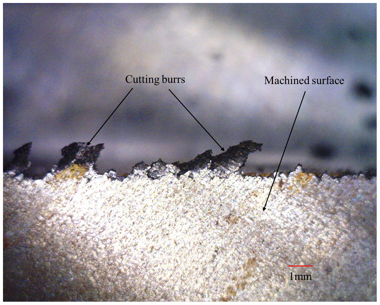
In the process of milling CGI, the height of the cutting burrs which appeared on the exit side was measured at the end of the tool life with the help of the toolmaker's microscope. The form of cutting burrs is plural form in this work. Figure 3 is the morphologies of cutting burrs. Due to the irregular shape of the cutting burr, the measurements have been repeated four times and the average value is determined for the final value.
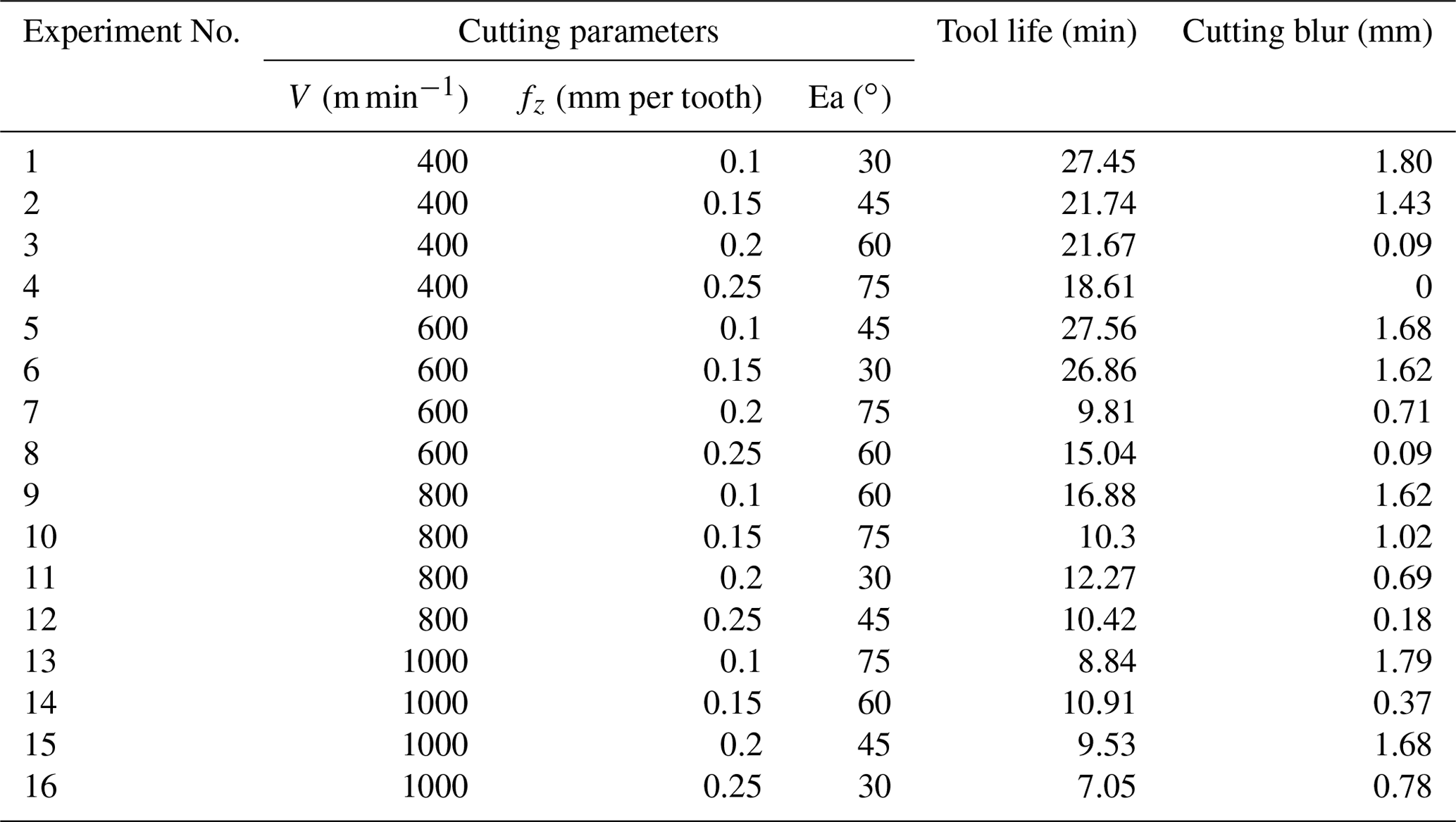
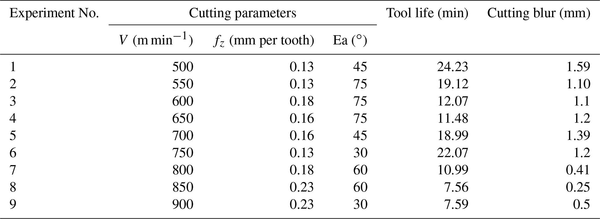
It is proved by experiment that the coated tool is the first choice in the cutting process of CGI in dry cutting conditions. During the high speed milling, three parameters need to be considered: cutting speed, feed rate and exit angle. As can be seen in Table 2, the cutting speed, feed rate and exit angle are set as four levels for training data, 400, 600, 800 and 1000 m min−1 for the cutting speed, 0.1, 0.15, 0.2 and 0.25 mm per tooth for feed rate and 30, 45, 60 and 75∘ for exit angle, respectively. For testing of the data set, the cutting speed and feed rate have nine and four different levels, respectively. Different exit angles put the cutting plate in a different position relative to the workpiece material, as shown in Fig. 4. The exit angle is obtained by Eq. (2),
where, Ea is the exit angle, M is the width of the workpiece material; R is the radius of the cutter, and d is the distance between the milling cutter axis and the workpiece central line.
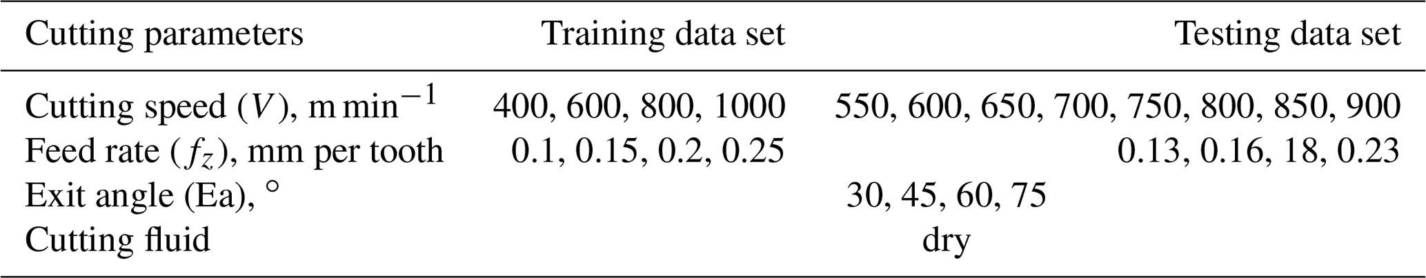
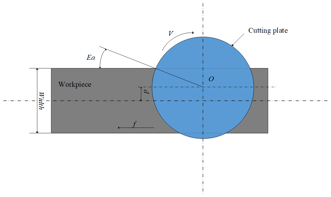
Figure 4The distribution circumstance of the cutting speed, the feed rate and the exit angle in the process of milling
4.1 ANFIS
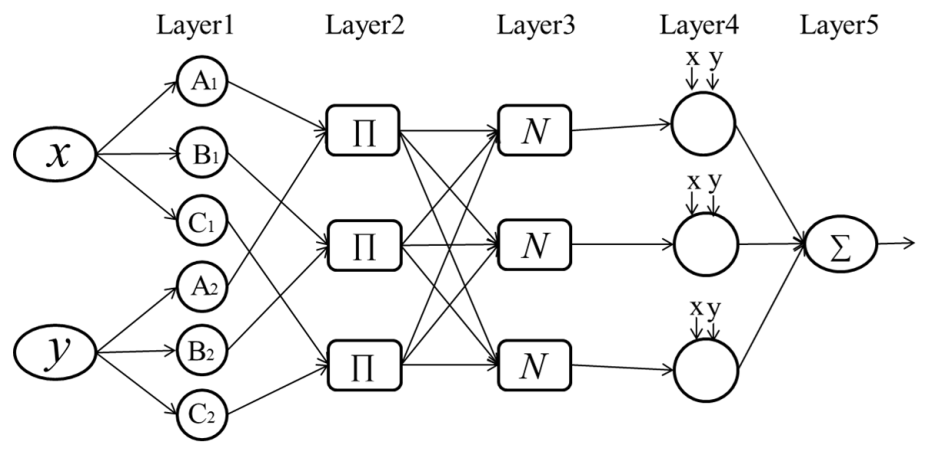
ANFIS, which combines fuzzy inference system and neural network, is proposed by Jang (1993), and the architecture of the ANFIS system is shown in Fig. 5. There are five layers in this inference system. The number of the nodes in each layer is determined according to the research requirement. Each node means a special function which accepts the previous layer signals and manipulates them to the output signals. Meantime, the ANFIS model has the rule base which is clarified as follows.
Rule 1: if x is the cutting speed A1, y is the feed rate B1 and z is the exit angle C1, then tool life and height of cutting burrs .
Rule 2: if x is the cutting speed A2, y is the feed rate B2 and z is the exit angle C2, then tool life and height of cutting burrs .
Then, the meaning of each layer in the ANFIS is described below.
Layer 1: The membership grade of a linguistic label is generated by each node “l” in this layer. These input numbers are real numbers and the output numbers are values of membership functions. The node function is,
where, x is called input value of the node, and Al is called linguistic variables.
The membership functions have many different forms, like triangular, bell-shaped, Gaussian, and so on. The Gaussian membership functions (MFs), adapted with minimum and maximum equal to 0 and 1, respectively, has the following formula:
where, the value of is the input, and cX,i, σX,i are the center parameter and standard deviation of Gaussian MF, respectively. These parameters are named as premise parameters. If these parameters' values are changed, the form of membership functions will be changed synchronously. In this layer, denotes the input of Layer 2.
Layer 2: This layer can calculate the firing strength for the third layer through multiplication. The function is shown as follows:
Layer 3: This layer is called the normalized layer where the normalized firing strengths are acquired through Eq. (6);
Layer 4: This layer is named as the adaptive layer. The formula is described bellow:
The parameters sl, fl, nl in this layer are called consequent parameters.
Layer 5: This layer is named as the output or defuzzification layer. The output is the final outcome, with the outcome defined as below:
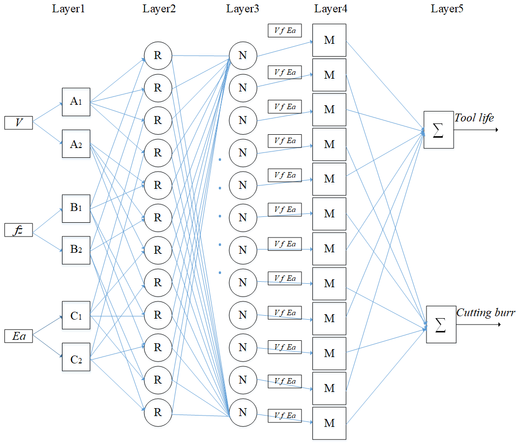
4.2 Improved ANFIS
The standard ANFIS mainly supports multiple inputs and single output mode. In order to make the ANFIS support multiple inputs multiple outputs mode, the structure of the ANFIS is modified as shown in Fig. 6. In this model, the inputs are cutting speed (V), feed rate (fz) and exit angle (Ea), and the outputs are tool life and height of cutting burr. There are 12 rules in this ANFIS and the number of membership function is 6.
4.3 ANFIS with optimization model
Based on Eqs. (3)–(8), ANFIS can predict the right output value when the premise parameters and the consequent parameters are optimized well. The optimization model can obtain the right parameters where the Root Mean Square Error (RMSE) is chosen for the fitness function. The equation can be expressed as follows,
where m denotes the number of training data, s(r)denotes the rth tool life, and p(r) is the rth prediction of ANFIS.
As can be seen from the ANFIS, through the RMSE and self-learning strategy, the premise parameters (cX,i, σX,i), and the consequent parameters (s, f, d, n) are determined. Also it can be seen that if the number of the membership functions is l and the number of rules is h, the total number of variables is (2l+4h) in this model.
Because the premise parameters and consequent parameters are unknown in ANFIS architecture, the aim of the self-learning method is to change the above parameters to match the training data. There are lots of self-learning ways introduced to optimize and establish the premise parameters and consequent parameters of ANFIS. The right learning methods should maintain the balance between prediction accuracy and computing power. After the specified number of iterations, the premise parameters and the consequent parameters can be optimized and stabilized. In this work, DE is proposed for its efficient, robust and easy to implement in finding the optimal premise parameters and consequent parameters of ANFIS.
4.4 Differential evolution algorithm
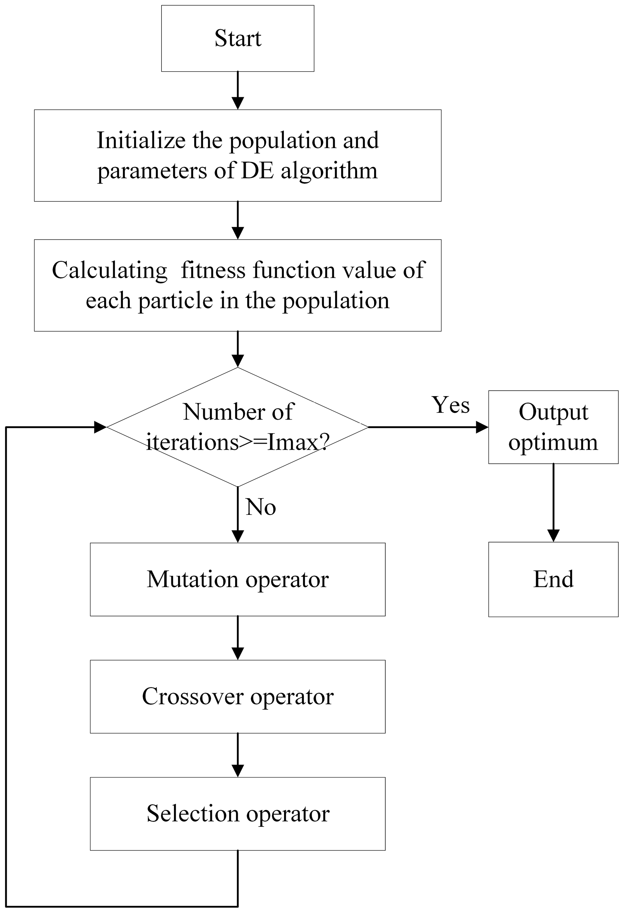
DE, proposed by Storn and Price (1995), is a heuristic random search algorithm based on group difference. Figure 7 shows the flowchart of the differential evolution algorithm. It can generate new different candidate solutions using the operators of mutation and crossover. By the selection operator, the best candidate solution is selected and enters the next loop operation up until the maximum iteration. Each candidate solution, as a vector defined as Xi,g, has many variables to solve the problem. At the beginning stage, the size of candidate solutions is determined and these candidate solutions form a population, symbolized by PX,g. The population is defined as:
where N denotes the number of candidate solutions, and i denotes the population index parameters of Xi,g. The index g represents the generation counter.
Each variable in the candidate solutions is randomly determined within a reasonable initial range. The values of Xi,g are determined as:
where the bi,L and bi,U are the lower and upper bounds of the i th value of the Xi,g. Rand (0, 1) means a uniformly distributed random number between 0 and 1.
After the initialization of the population, the next step is the mutation operator. The mutation operator forms an intermediary population, Pv,g of N mutant vectors, Vi,g.
Different mutation strategies are defined in determining Vi,g and it mainly depends on the choice of the three different individuals Xa,g, Xc,g, and Xb,g. These strategies are shown in the follows:
where, S denotes the different degree of variation iterating from g to the maximum number of iterations gmax. a, b and c belong to index parameters of D dimensions and they are not equal to each other. F is a scale factor. The value of F is changed with increase of the number of iterations which can maintain the diversity of the population.
In order to further improve the diversity of the population, the crossover operator is used to form the trial population, PU,g of N trial vectors, Ui,g.
Binomial and exponential are two kinds of crossover scheme. In this study, the binomial crossover is adopted due to being widely used. The binomial crossover operator is shown as follows:
where, Cr belongs to the range (0, 1), is the crossover rate and its value can control parts of parameter values that it inherits from the value of the mutant. Rand j (0, 1) is a random number that generate with the jth parameter. jrand is a randomly distributed integer in the range [1, D]. If Ui,g is outside the boundary, its value will be re-restricted within the allowable range.
The last step is the selection operator and it determines which vector, Xi,g or Ui,g, can enter the next generation. As the vectors Xi,g and Ui,g have the objective function, the vector with the lower value of the objection function is selected through the selection operator. The selection operator is given as:
The settings of the scale factor F and the crossover rate Cr determine the performance of the DE. In order to choose the right F and Cr values, Liu and Lampinen (2002) suggested , while Zielinski et al. (2006) demonstrated that in many cases, values of F (0.6, 1) and Cr (0.6, 1) can make DE yield a better performance. Zaharie (2002) modified the DE by multiplying F by a standardized random variable. Based on these studies, Cr=0.9 was selected for the DE, and F was limited between 0 and 1 while changing with an increase in the number of iterations.
After high speed milling process on CGI, the training data set and the testing data set are collected and shown in the Tables 3 and 4. Before training the DE-ANFIS model, all of the experimental data needed to be normalized in the range (0, 4) with the formula shown below:
where, Xi and Yi are the raw data and the normalized data respectively.
5.1 Prediction ability of DE-ANFIS
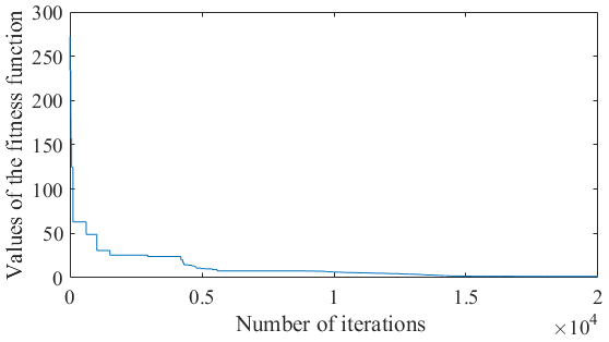
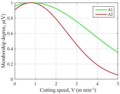
The DE-ANFIS is programed and running in the MATLAB software. Meanwhile, training error goal is set as 0. During DE learning stage, each randomly distributed candidate solution is self-mutated and crossed with each other to achieve the optimal solution of fitness function. The Gaussian membership functions (GMFs) which calculate the membership degree for the inputs are used and labeled as A1, A2, B1, B2, C1, C2 regions for each input. After DE learning, the premise parameters and consequent parameters of ANFIS tend towards stability. Figure 8 shows the relationship between fitness function and iterations. It is obvious that the fitness function gradually converges to 0 with an increase of iterations. The final GMFs of V, fz and Ea are shown in Figs. 9, 10, and 11.
The comparison of the measured and predicted values of tool life and height of the cutting burrs for training data are shown in Table 3. After the training, the predictive capability of the DE-ANFIS system is tested using a testing data set. Table 5 shows the predicted values of tool life and cutting burr by the developed DE-ANFIS system. To evaluate the performance of DE-ANFIS model, the Root Mean Squared Error (RMSE), the mean absolute error (MAE) and coefficient of correlation (R2) were calculated using Eqs. (23)–(26).
where, n, xi and xp are number of datasets, the value of the ith measured and predicted output.
Table 5The measured and predicted values of tool life and heights of cutting burr for training data set.
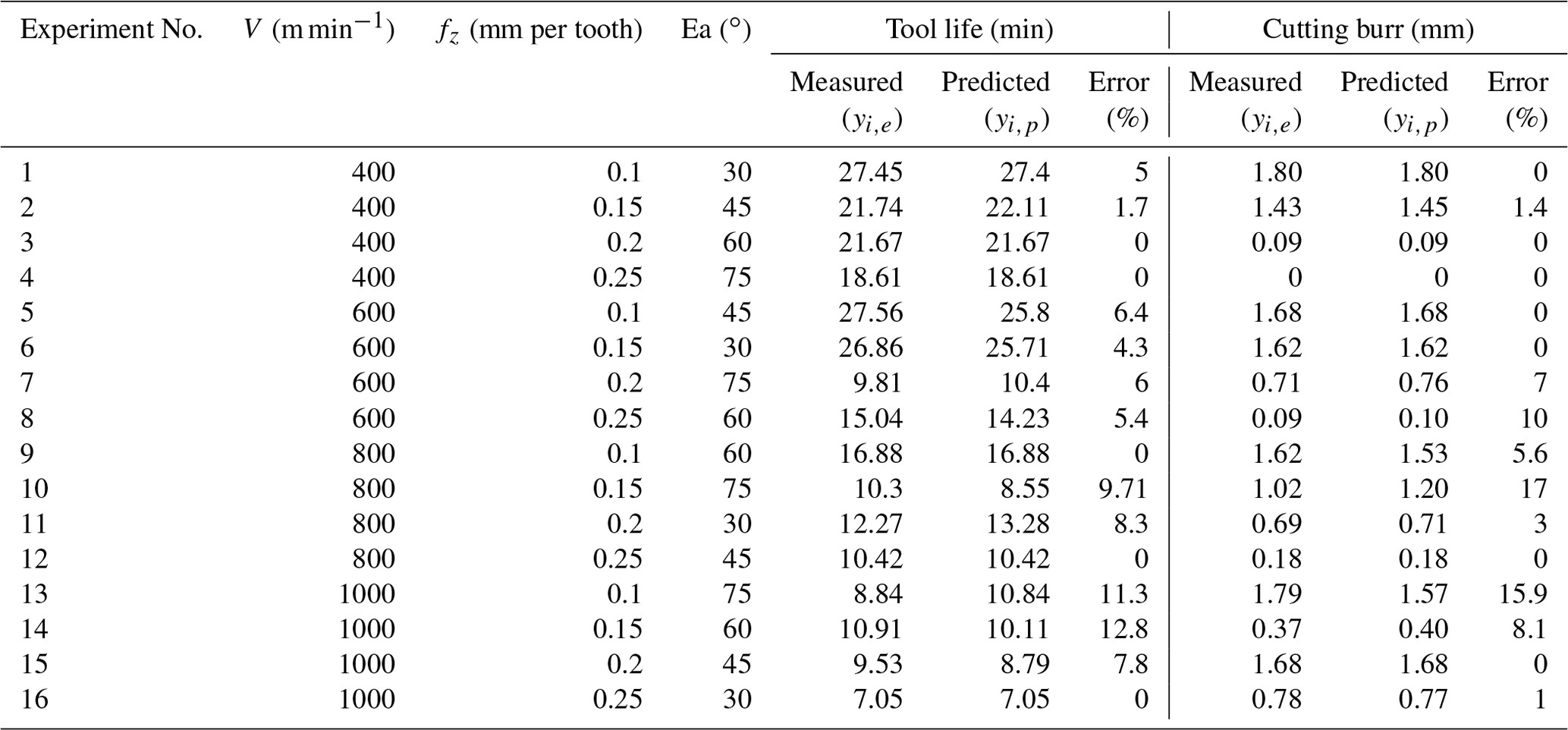
Table 6The measured and predicted values of tool life and heights of cutting burr for testing data set.
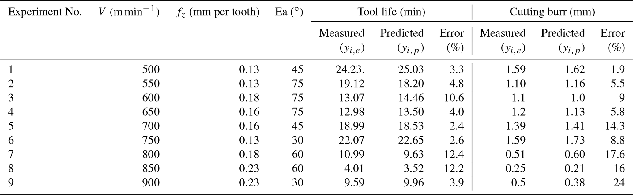
The MAE, RMES and R2 of the predicted tool life shown in Table 4 are 6.24, 0.85 and 0.98, respectively. As for cutting burrs, the MAE, RMSE and R2 are found as 11.43, 0.08 and 0.92, respectively. It can be seen that the training of ANFIS with DE learning algorithm can provide pretty high prediction accuracy for tool life and height of the cutting burrs.
The relationship between the predicted values and measured values of tool life and cutting burrs for testing data is shown in Figs. 12 and 13 in forms of scatter diagrams. Figure 12 shows the predicted values of tool life are uniformly distributed near the line. That means the predicted values of tool life are not far from the actual values. The errors between the predicted values and the measured values may be predominately attributed to the typical randomness of the milling process. In addition, the violent vibration of CNC machine also affects the accuracy of predicted tool life. In Fig. 13, the cutting burr distribution is more scattered than that of the distribution in Fig. 12. It can be seen from Table 6 and Fig. 13, the prediction of cutting burr is not as accurate as the prediction of tool life. The prediction error of an individual cutting burr can even reach up to 20 %. The emergence of this phenomenon is mainly related to the wear state of the cutting tool. With the increasing cutting speed, the generation of hot cracks on tool flack can increase the probability of tool tipping. The occurrence of tool tipping on tool flack makes the deformation of cutting burr more serious than a normal wear tool. Generally, the DE-based ANFIS model still gains a satisfactory performance aiming at the prediction of height of the cutting burrs.
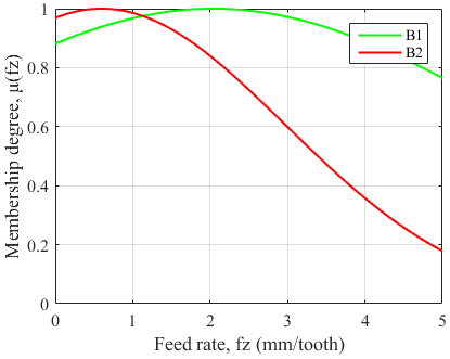
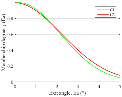
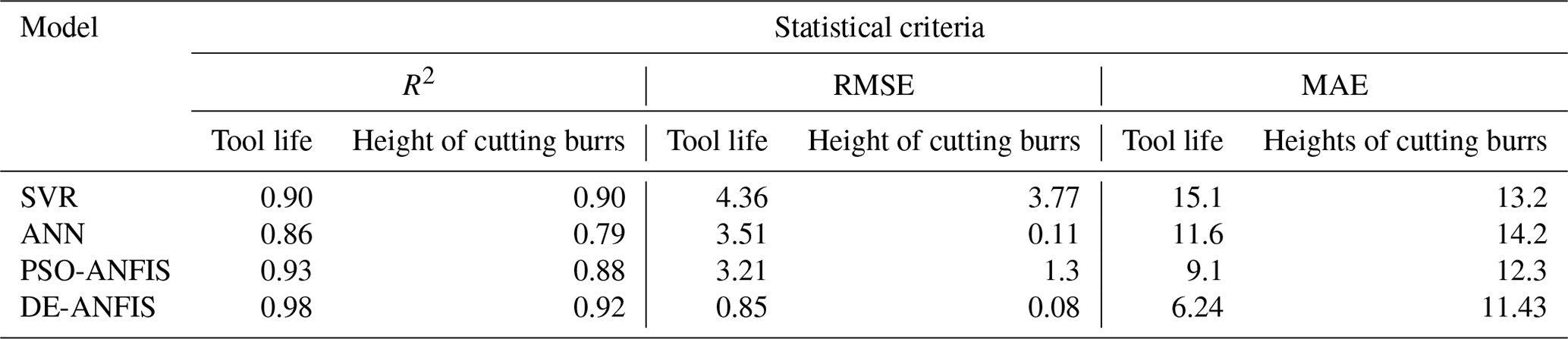
Table 8Analysis of variance results for tool life and height of cutting burrs.
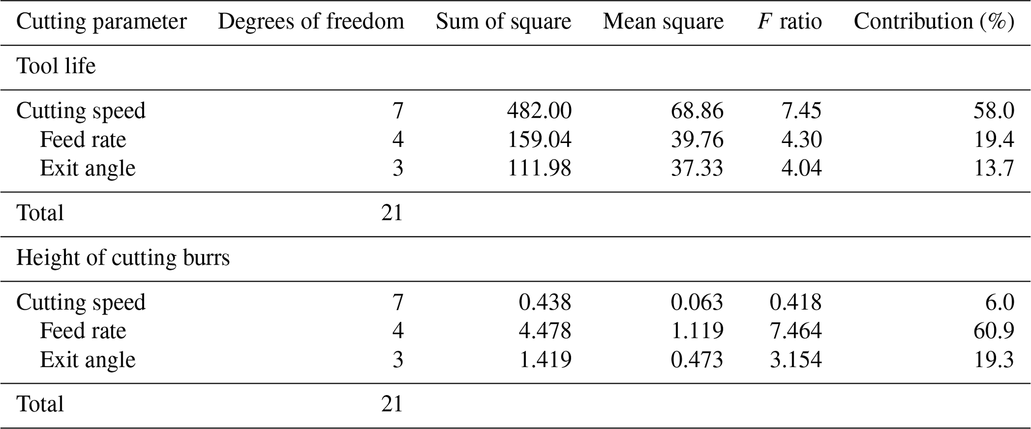
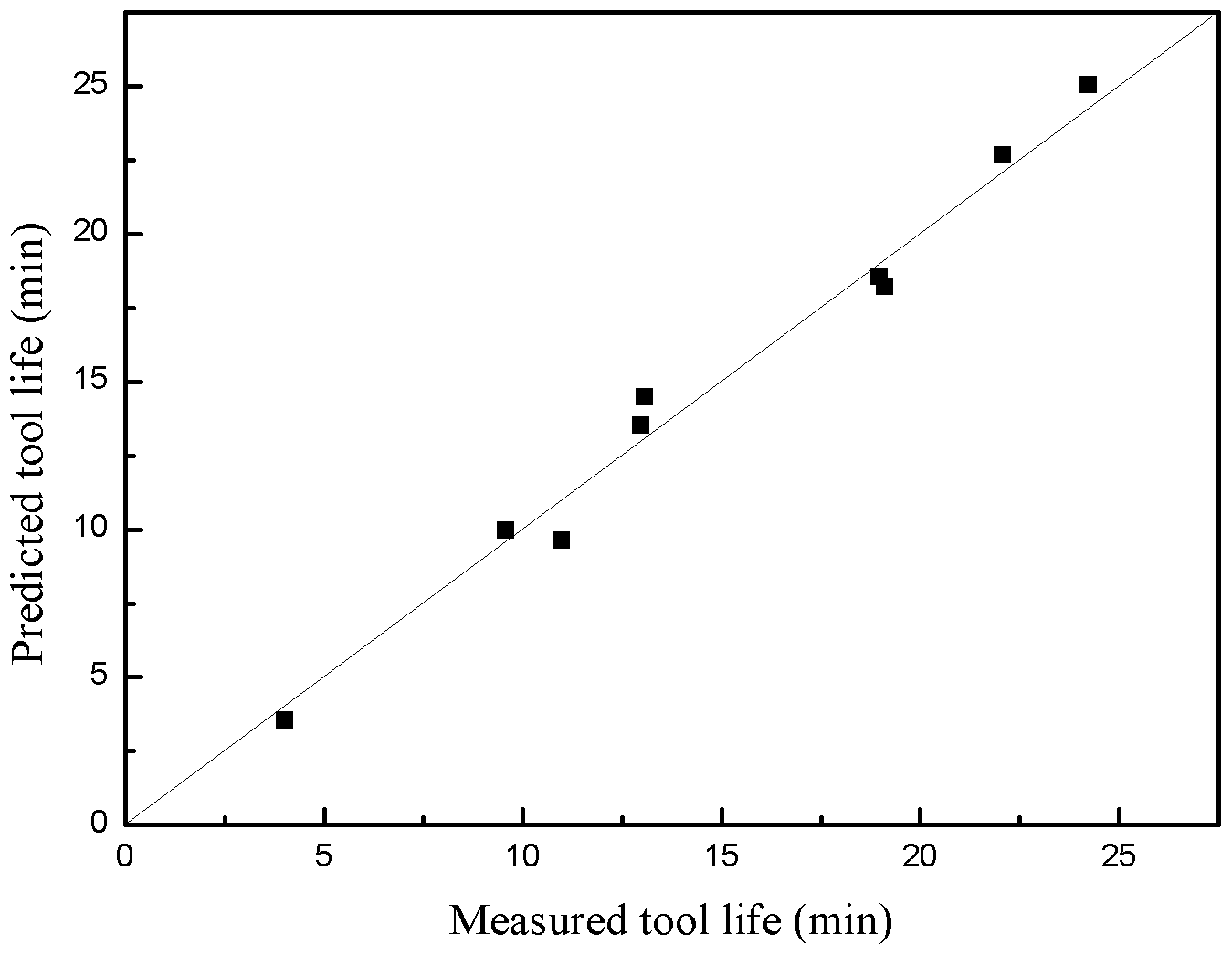
Figure 12Scatter diagram of measured tool life and predicted tool life for the testing data set.
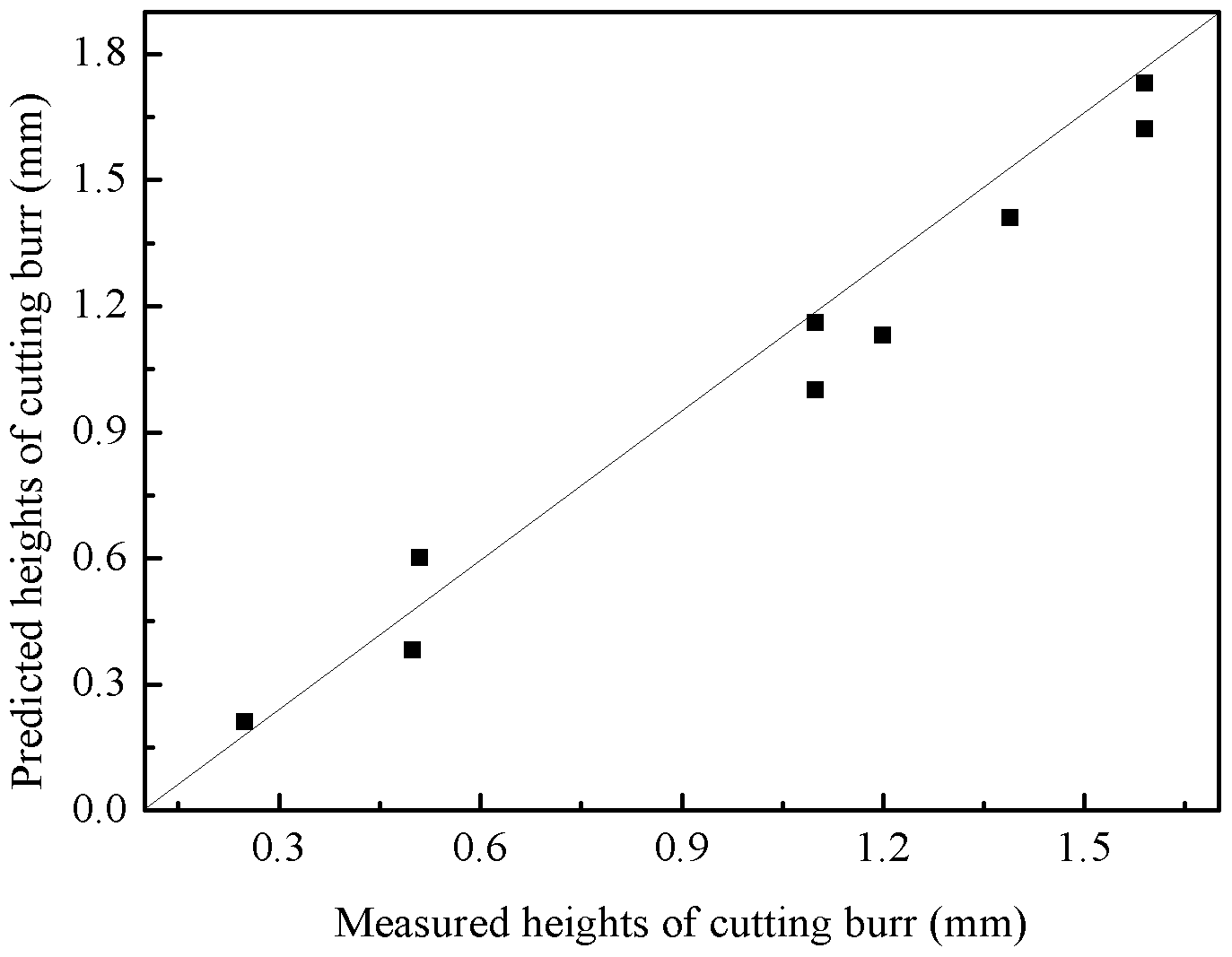
Figure 13Scatter diagram of measured cutting burr and predicted cutting burr for the testing data set.
Figures 14 and 15 compare the predicted values and measured values of tool life and cutting burr for a testing data set. As can be seen from Figs. 14 and 15, it can be seen that the predicted and measured values are close to each other and show the same trend. The analysis of Figs. 12, 13, 14 and 15 indicate that the DE-based ANFIS system can provide an adequately accuracy rate when milling CGI with high cutting speed.
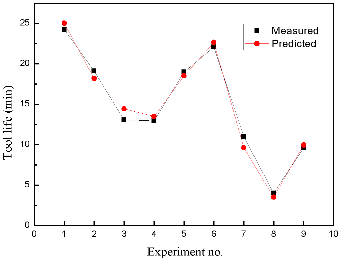
Figure 14The diagram of measured tool life and predicted tool life for the testing data set.
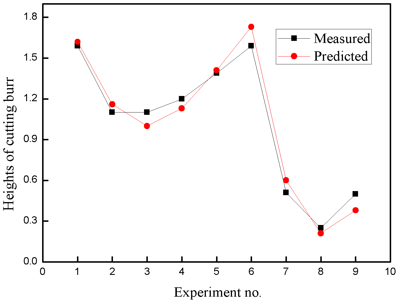
Figure 15The diagram of measured cutting burr and predicted cutting burrs for the testing data set.
5.2 Comparison with other prediction models
In this work, DE-ANFIS model is proposed to estimate tool life and cutting burr. For comparison aims, ANFIS with particle swarm optimization (PSO-ANFIS), artificial neural network (ANN) and support vector machines (SVM) models were also proposed. PSO-ANFIS is a model that its parameters are optimized with PSO algorithm. To obtain a good PSO-ANFIS model, the parameters of PSO algorithm are adjusted with a trial-and error procedure. The structure of PSO-ANFIS model is the same as the DE-ANFIS model where there are 12 rules and the number of GMFs is 6. In order to develop the PSO-ANFIS, ANN and SVM models in this work, the same training and testing datasets considering in DE-ANFIS was used. It should be mentioned that MATLAB 2015 was used to construct the PSO-ANFIS model. Apart from the PSO-ANFIS and DE-ANFIS models, ANN and SVM models which are widely used methods for solving different engineering problems were utilized for prediction of tool life and height of cutting burrs.
In the second step, for checking the performance capacity of the models, the RMSE, MAE and R2 were used. It can be shown from Table 7 that the DE-ANFIS model can predict tool life and cutting burr better than PSO-ANFIS, ANN and SVM models. The results demonstrate that predictive capability of DE-ANFIS model is more accurate in comparison with PSO-ANFIS, ANN and SVM models.
5.3 Sensitivity analysis
In order to obtain the most influential factors on the tool life and cutting burr, Analysis of Variance (ANOVA) was performed in this paper. Table 8 shows the tool life is sensitive to, in descendent order, cutting speed, feed rate and exit angle, and cutting burr is sensitive to feed rate, exit angle and cutting speed. During the milling process, cutting speed is the main factor that affects the tool life. High cutting speed can generate a massive of cutting heat, and meantime increase the cutting force which can accelerate tool flank wear. The rapid tool flank wear reduces tool life. Feed rate and exit angle have little effect on tool life. Hence, it's better to adopt low cutting speed, high feed rate and small exit angle to prolong tool life and enhance cutting efficiency. As for cutting burrs, feed fate is the main factor that affects the height of cutting burrs as can be seen from Tables 3 and 8. In order to reduce the height of cutting burrs, the high feed rate and small exit angle were adopted in this work. In Table 8, Cutting speed has little effect on the height of cutting burrs, and its value can be determined according to process requirements. Therefore, to prolong tool life and reduce the height of cutting burrs, low cutting speed, high feed rate and small exit angle is necessary in milling process of CGI in the present research work.
In this paper, a new DE-ANFIS system was proposed to accurately predict tool life and height of the cutting burrs in high speed milling of CGI. The DE-ANFIS model is an MIMO system where the inputs are cutting speed, feed rate, and exit angle, and the outputs are tool life and height of the cutting burrs. DE can determine the right premise and consequent parameters of ANFIS. After training the ANFIS stage, the testing data is used to validate the performance of DE-ANFIS. In order to examine the accuracy of tool life and height of cutting burr predictions by DE-ANFIS, PSO-ANFIS, ANN and SVM models, three statistical indices including R2, RMSE and MAE have been used. Comparing the values predicted by the models indicated that the performance of the DE-ANFIS model was better than the PSO-ANFIS, ANN, and SVM models. Results showed that MAE values in the DE-ANFIS, PSO-ANFIS, ANN and SVM models were 6.24, 9.1, 11.6 and 15.1 for tool life, and the MAE values of height of cutting burrs are 11.43, 12.3, 14.2 and 13.2 respectively. Based on the ANOVA, the results show that the most effect on the tool life and height of cutting burrs are cutting speed and feed rate respectively.
The prediction ability makes DE-ANFIS a powerful tool for the milling process, and thus the estimation of tool life and height of the cutting burrs under different cutting parameters can be known in advance. Consequently, efficient processing has been improved accordingly through the proposed approach. The DE learning algorithm, a global optimization algorithm, can considerably reduce the computational time and manufacturing cost for milling. Traditional selecting of cutting parameters by trial is replaced by the DE learning algorithm. Thus, a better product quality or high productivity with a low cost can be obtained through DE-ANFIS model.
All the data used in this paper can be obtained by request from the corresponding author.
CH and LX suggested the overall concept of this paper. LX, RS, YL and CL completed the experiment together. HZ, HL and JW verified the proposed artificial model with the experiments and supervised the whole project.
The authors declare that they have no conflict of interest.
This research has been supported by the National Natural Science Foundation of China (grant nos. 51675312, 51675313).
This paper was edited by Xichun Luo and reviewed by yukui cai and one anonymous referee.
Chern, G. L.: Experimental observation and analysis of burr formation mechanisms in face milling of aluminum alloys, Int. J. Mach. Tool. Manu., 46, 1517–1525, https://doi.org/10.1016/j.ijmachtools.2005.09.006, 2006.
Chuang, C., Singh, D., Kenesei, P., Jon, Almer, J., Hryn, J., and Huff, R.: Application of X-ray computed tomography for the characterization of graphite morphology in compact-graphite iron, Mater. Charact., 141, 442–449, https://doi.org/10.1016/j.matchar.2016.08.007, 2018.
Dong, M. G. and Wang, N.: Adaptive network-based fuzzy inference system with leave-one-out cross-validation approach for prediction of surface roughness, Appl. Math. Model., 35, 1024–1035, https://doi.org/10.1016/j.apm.2010.07.048, 2011.
Gabaldo, S., Diniz, A. E., Andrade, C. L. F., and Guesser, W. L.: Performance of carbide and ceramic tools in the milling of compact graphite iron-CGI, J. Braz. Soc. Mech. Sci., 32, 511–517, https://doi.org/10.1590/S1678-58782010000500011, 2010.
Gill, S. S., Singh, R., Singh, J., and Singh, H.: Adaptive neuro-fuzzy inference system modeling of cryogenically treated AISI M2 HSS turning tool for estimation of flank wear, Expert Syst. Appl., 39, 4171–4180, https://doi.org/10.1016/j.eswa.2011.09.117, 2012.
Jang, S. R.: ANFIS: adaptive-network-based fuzzy inference system, IEEE Trans. Syst. Man Cyb., 23, 665–685, https://doi.org/10.1109/21.256541, 1993.
Lee, K. M., Hsu, M. R., Chou, J. H., and Guo, C. Y.: Improved differential evolution approach for optimization of surface grinding process, Expert Syst. Appl., 38, 5680–5686, https://doi.org/10.1016/j.eswa.2010.10.067, 2011.
Liu, J. H. and Lampinen, J.: A fuzzy adaptive differential evolution algorithm, IEEE Region 10 Conference on Computers., 606–611, https://doi.org/10.1109/TENCON.2002.1181348, 2002.
Mehmet, A., Cihan, K., Mehmet, U., Abdulkadir, C., and Mehmet A. Ç.: Prediction of surface roughness and cutting zone temperature in dry turning processes of AISI304 stainless steel using ANFIS with PSO learning, Int. J. Adv. Manuf. Tech., 957–967, https://doi.org/10.1007/s00170-012-4540-2, 2013.
Ming, C., Jiang, L., Guo, G. Q., and An, Q. L.: Experimental and FEM Study of Coated and Uncoated Tools Used for Dry Milling of Compacted Graphite Cast Iron, Transactions of Tianjin University, 17, 235–241, https://doi.org/10.1007/s12209-011-1609-1, 2011.
Olvera, O. and Barrow, G.: Influence of exit angle and tool nose geometry on burr formation in face milling operations, Proc. Inst. Mech. Eng. B J. Eng. Manuf., 212, 59–72, https://doi.org/10.1243/0954405981515509, 1998.
Qiu, Y., Pang, J. C., Zou, C. L., Zhang, M. X., Li, S. X., and Zhang, Z. F.: Fatigue strength model based on microstructures and damage mechanism of compacted graphite iron, Mat. Sci. Eng. A-Struct., 724, 324–329, https://doi.org/10.1016/j.msea.2018.03.110, 2018.
Storn, R. and Price, K.: Differential evolution: A simple and efficient adaptive scheme for global optimization over continuous spaces, University of California, Berkeley, 1995.
Su, R., Huang, C. Z., Zou, B., Liu, G. L., Zhan, Liu, Z. Q., Liu, Y., and Li, C. W.: Study on cutting burr and tool failure during high-speed milling of compacted graphite iron by the coated carbide tool, Int. J. Adv. Manuf. Tech., 9, 1–11, https://doi.org/10.1007/s00170-017-1573-6, 2018.
Varun, N., Gustav, G., Jacek, K., and Lars, N.: Machinability of Compacted Graphite Iron (CGI) and Flake Graphite Iron (FGI) with Coated Carbide, Int. J. of Machining and Machinability of Materials, 13, 67–90, https://doi.org/10.1504/IJMMM.2013.051909, 2013.
Wang, G. F., Xie, Q. L., and Zhang, Y. C.: Tool condition monitoring system based on support vector machine and differential evolution optimization, P. I. Mech. Eng., 231, 805–813, https://doi.org/10.1177/0954405415619871, 2017.
Yang, S. H., Natarajan, U., Sekar, M., and Palani, S.: Prediction of surface roughness in turning operations by computer vision using neural network trained by differential evolution algorithm, Int. J. Adv. Manuf. Tech., 51, 965–971, https://doi.org/10.1007/s00170-010-2668-5, 2010.
Zaharie, D.: Critical values for control parameters of differential evolution algorithm, in: Proceedings MENDEL, 8th MENDEL International Conference on Soft Computing, Brno, Czech Republic, 62–67, 2002.
Zielinski, K., Weitkemper, P., Laur, R., and Kammeyer, K. D.: Parameter Study for Differential Evolution Using a Power Allocation Problem Including Interference Cancellation, IEEE Congress on Evolutionary Computation, CEC 2006, Vancouver, BC, Canada, https://doi.org/10.1109/CEC.2006.1688533, 2006.